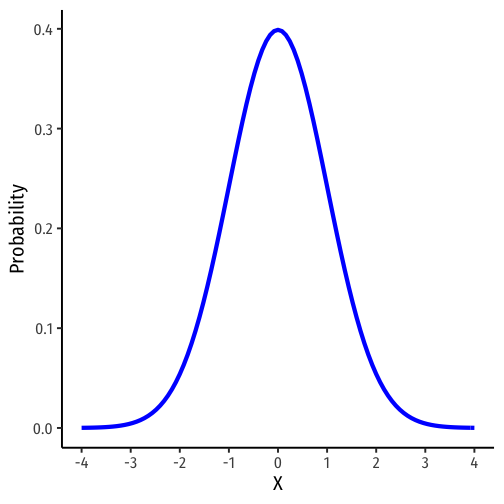
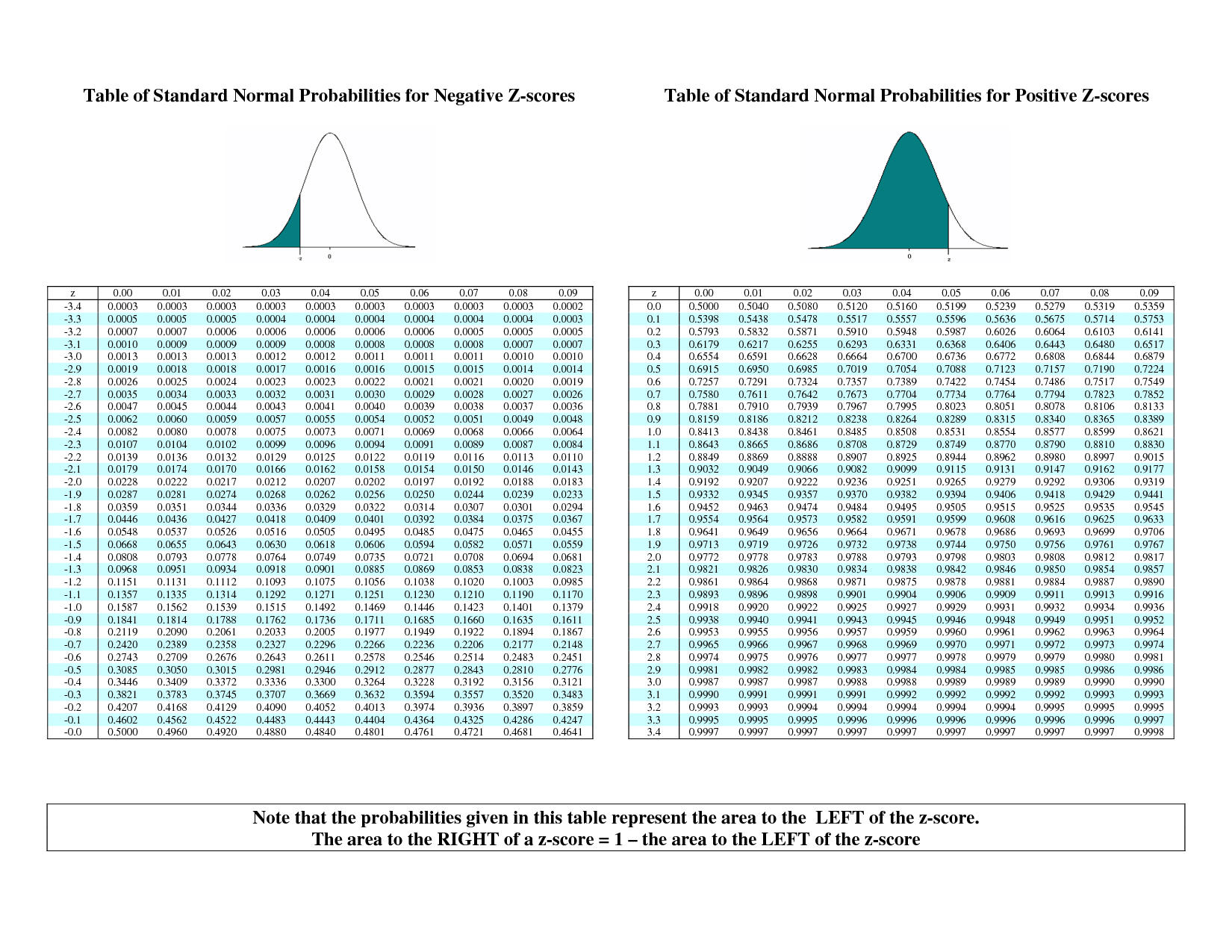
2.1 — Random Variables & Distributions

# 2.1 — Random Variables & Distributions
## ECON 480 • Econometrics • Fall 2020
### Ryan Safner Assistant Professor of Economics <a href="mailto:safner@hood.edu">safner@hood.edu</a> <a href="https://github.com/ryansafner/metricsF20">ryansafner/metricsF20</a> <a href="https://metricsF20.classes.ryansafner.com"> metricsF20.classes.ryansafner.com</a>

---

---

# Experiments

- An .hi-purple[experiment] is any procedure that can (in principle) be repeated infinitely and has a well-defined set of outcomes

]
]

---

# Random Variables

- A .hi-purple[random variable (RV)] takes on values that are unknown in advance, but determined by an experiment

- A numerical summary of a random outcome

]
]

---

# Random Variables: Notation

- Random variable `$X$` takes on individual values `$(x_i)$` from a set of possible values

- Often capital letters to denote RV's
    - lowercase letters for individual values

.content-box-green[
.green[**Example**]: Let `$X$` be the number of Heads from 10 coin flips. `$\quad x_i \in \{0, 1, 2,...,10\}$`
]

---

---

# Discrete Random Variables

- A .hi[discrete random variable]: takes on a finite/countable set of possible values

.content-box-green[
.green[**Example**]: Let `$X$` be the number of times your computer crashes this semester.red[1], `$x_i \in \{0, 1, 2, 3, 4\}$`
]

]

---

# Discrete Random Variables: Probability Distribution

.pull-left[
- .hi[Probability distribution] of a R.V. fully lists all the possible values of `$X$` and their associated probabilities
]

| `$x_i$`  | `$P(X=x_i)$` |
|--------|------------|
| 0      | 0.80       |
| 1      | 0.10       |
| 2      | 0.06       |
| 3      | 0.03       |
| 4      | 0.01       |

]

---

# Discrete Random Variables: pdf

.pull-left[
.hi[Probability distribution function (pdf)] summarizes the possible outcomes of `$X$` and their probabilities

- Notation: `$f_X$` is the pdf of `$X$`:

`$$f_X=p_i, \quad i=1,2,...,k$$`

- For any real number `$x_i$`, `$f(x_i)$` is the probablity that `$X=x_i$`

]

| `$x_i$`  | `$P(X=x_i)$` |
|--------|------------|
| 0      | 0.80       |
| 1      | 0.10       |
| 2      | 0.06       |
| 3      | 0.03       |
| 4      | 0.01       |

]

- What is `$f(0)$`?

- What is `$f(3)$`?

---

# Discrete Random Variables: pdf Graph

```r
crashes<-tibble(number = c(0,1,2,3,4),
 prob = c(0.80, 0.10, 0.06, 0.03, 0.01))

ggplot(data = crashes)+
  aes(x = number,
      y = prob)+
  geom_col(fill="#0072B2")+
  labs(x = "Number of Crashes",
       y = "Probability")+
    theme_classic(base_family = "Fira Sans Condensed",
           base_size=20)
```

]
]
.pull-right[

<img src="2.2-slides_files/figure-html/unnamed-chunk-2-1.png" width="504" />
]

---

# Discrete Random Variables: cdf

.pull-left[
.hi[Cumulative distribution function (pdf)] lists probability `$X$` will be *at most* (less than or equal to) a given value `$x_i$`

- Notation: `$F_X=P(X \leq x_i)$`

]

| `$x_i$`  | `$f(x)$` | `$F(x)$` |
|--------|--------|--------|
| 0      | 0.80   | 0.80   |
| 1      | 0.10   | 0.90   |
| 2      | 0.06   | 0.96   |
| 3      | 0.03   | 0.99   |
| 4      | 0.01   | 1.00   |

]

- What is the probability your computer will crash *at most* once, `$F(1)$`?

- What about three times, `$F(3)$`?

---

# Discrete Random Variables: cdf Graph

```r
crashes<-crashes %>%
 mutate(cum_prob = cumsum(prob))

crashes
```

```
## # A tibble: 5 x 3
## number prob cum_prob
## <dbl> <dbl> <dbl>
## 1 0 0.8 0.8 
## 2 1 0.1 0.9 
## 3 2 0.06 0.96
## 4 3 0.03 0.99
## 5 4 0.01 1
```

```r
ggplot(data = crashes)+
  aes(x = number,
      y = cum_prob)+
  geom_col(fill="#0072B2")+
  labs(x = "Number of Crashes",
       y = "Probability")+
    theme_classic(base_family = "Fira Sans Condensed",
           base_size=20)
```

]
]

<img src="2.2-slides_files/figure-html/unnamed-chunk-5-1.png" width="504" />
]

---

---

# Expected Value of a Random Variable

- .hi[Expected value] of a random variable `$X$`, written `$E(X)$` (and sometimes `$\mu)$`, is the long-run average value of `$X$` "expected" after many repetitions

`$$E(X)=\sum^k_{i=1} p_i x_i$$`

- `$E(X)=p_1x_1+p_2x_2+ \cdots +p_kx_k$`

- A **probability-weighted average** of `$X$`, with each `$x_i$` weighted by its associated probability `$p_i$`

- Also called the .hi["mean"] or .hi["expectation"] of `$X$`, always denoted either `$E(X)$` or `$\mu_X$`

---

# Expected Value: Example I

.content-box-green[
.green[**Example**]: Suppose you lend your friend $100 at 10% interest. If the loan is repaid, you receive $110. You estimate that your friend is 99% likely to repay, but there is a default risk of 1% where you get nothing. What is the expected value of repayment?

]

---

# Expected Value: Example II

Let `$X$` be a random variable that is described by the following pdf:

| `$x_i$`  | `$P(X=x_i)$` |
|--------|------------|
| 1      | 0.50       |
| 2      | 0.25       |
| 3      | 0.15       |
| 4      | 0.10       |

Calculate `$E(X)$`.

---

# The Steps to Calculate E(X), Coded

```r
# Make a Random Variable called X
X<-tibble(x_i=c(1,2,3,4), # values of X
 p_i=c(0.50,0.25,0.15,0.10)) # probabilities

X %>%
  summarize(expected_value = sum(x_i*p_i))
```

```
## # A tibble: 1 x 1
## expected_value
## <dbl>
## 1 1.85
```

---

# Variance of a Random Variable

- The .hi[variance] of a random variable `$X$`, denoted `$var(X)$` or `$\sigma^2_X$` is:

`$$\begin{align*}\sigma^2_X &= E[(x_i-\mu_X)^2]\\
&=\sum_{i=1}^n(x_i-\mu_X)^2p_i\\ \end{align*}$$`

- This is the .hi-purple[expected value of the squared deviations from the mean]
    - i.e. the probability-weighted average of the squared deviations

---

# Standard Deviation of a Random Variable

- The .hi[standard deviation] of a random variable `$X$`, denoted `$sd(X)$` or `$\sigma_X$` is:

`$$\sigma_X=\sqrt{\sigma_X^2}$$`

---

# Standard Deviation: Example I

| `$x_i$`  | `$P(X=x_i)$` |
|--------|------------|
| 0      | 0.80       |
| 1      | 0.10       |
| 2      | 0.06       |
| 3      | 0.03       |
| 4      | 0.01       |

---

# The Steps to Calculate sd(X), Coded I

```r
# get the expected value 
crashes %>%
  summarize(expected_value = sum(number*prob))
```

```
## # A tibble: 1 x 1
## expected_value
## <dbl>
## 1 0.35
```

```r
# save this for quick use
exp_value<-0.35

crashes_2 <- crashes %>%
 select(-cum_prob) %>% # we don't need the cdf
 # create new columns
 mutate(deviations = number - exp_value, # deviations from exp_value
 deviations_sq = deviations^2,
 weighted_devs_sq = prob * deviations^2) # square deviations
```

---

# The Steps to Calculate sd(X), Coded II

```r
# look at what we made
crashes_2
```

```
## # A tibble: 5 x 5
## number prob deviations deviations_sq weighted_devs_sq
## <dbl> <dbl> <dbl> <dbl> <dbl>
## 1 0 0.8 -0.35 0.122 0.0980
## 2 1 0.1 0.65 0.423 0.0423
## 3 2 0.06 1.65 2.72 0.163 
## 4 3 0.03 2.65 7.02 0.211 
## 5 4 0.01 3.65 13.3 0.133
```

---

# The Steps to Calculate sd(X), Coded III

```r
# now we want to take the expected value of the squared deviations to get variance
crashes_2 %>%
  summarize(variance = sum(weighted_devs_sq), # variance
            sd = sqrt(variance)) # sd is square root
```

```
## # A tibble: 1 x 2
## variance sd
## <dbl> <dbl>
## 1 0.648 0.805
```

---

# Standard Deviation: Example II

.content-box-green[
.green[**Example**]: What is the standard deviation of the random variable we saw before?
]

| `$x_i$`  | `$P(X=x_i)$` |
|--------|------------|
| 1      | 0.50       |
| 2      | 0.25       |
| 3      | 0.15       |
| 4      | 0.10       |

Hint: you already found it's expected value.

---

---

# Continuous Random Variables

- .hi[Continuous random variables] can take on an uncountable (infinite) number of values

- So many values that the probability of any specific value is infinitely small:
`$$P(X=x_i)\rightarrow 0$$`

- Instead, we focus on a *range* of values it might take on

]

---

# Continuous Random Variables: pdf I

.pull-left[
.hi[Probability *density* function (pdf)] of a continuous variable represents the probability between two values as the area under a curve

- The total area under the curve is 1

- Since `$P(a)=0$` and `$P(b)=0$`, `$P(a<X<b)=P(a \leq X \leq b)$`

- See [today's class notes](/class/2.2-class) for how to graph math/stats functions in `ggplot`!
]

]

---

# Continuous Random Variables: pdf II

- FYI using calculus:

$$P(a \leq X \leq b) = \int_a^b f(x) dx $$

- Complicated: software or (old fashioned!) probability tables to calculate

]

]

---

# Continuous Random Variables: cdf I

- The .hi[cumulative density function (cdf)] describes the area under the pdf for all values less than or equal to (i.e. to the left of) a given value, `$k$`

`$$P(X \leq k)$$`

]

---

# Continuous Random Variables: cdf II

- Note: to find the probability of values *greater* than or equal to (to the right of) a given value `$k$`:

`$$P(X \geq k)=1-P(X \leq k)$$`

---

---

# The Normal Distribution I

- The .hi[Gaussian] or .hi[normal distribution] is the most useful type of probability distribution

$$ X \sim N(\mu,\sigma)$$

- Continuous, symmetric, unimodal, with mean `$\mu$` and standard deviation `$\sigma$`

]

]

---

# The Normal Distribution II

- FYI: The pdf of `$X \sim N(\mu, \sigma)$` is 
`$$P(X=k)=	\frac{1}{\sqrt{2\pi \sigma^2}}e^{-\frac{1}{2}\big(\frac{(k-\mu)}{\sigma}\big)^2}$$`

- **Do not try and learn this**, we have software and (previously tables) to calculate pdfs and cdfs

]

]

---

# The 68-95-99.7 Rule

- .hi[68-95-99.7% empirical rule]: for a normal distribution:
]

<img src="2.2-slides_files/figure-html/unnamed-chunk-17-1.png" width="504" />
]

---

# The 68-95-99.7 Rule

- .hi[68-95-99.7% empirical rule]: for a normal distribution:

- `$P(\mu-1\sigma \leq X \leq \mu+1\sigma) \approx$` 68%

]

<img src="2.2-slides_files/figure-html/unnamed-chunk-18-1.png" width="504" />
]

---

# The 68-95-99.7 Rule

- .hi[68-95-99.7% empirical rule]: for a normal distribution:

- `$P(\mu-1\sigma \leq X \leq \mu+1\sigma) \approx$` 68%

- `$P(\mu-2\sigma \leq X \leq \mu+2\sigma) \approx$` 95%

]

<img src="2.2-slides_files/figure-html/unnamed-chunk-19-1.png" width="504" />
]

---
# The 68-95-99.7 Rule

- .hi[68-95-99.7% empirical rule]: for a normal distribution:

- `$P(\mu-1\sigma \leq X \leq \mu+1\sigma) \approx$` 68%

- `$P(\mu-2\sigma \leq X \leq \mu+2\sigma) \approx$` 95%

- `$P(\mu-3\sigma \leq X \leq \mu+3\sigma) \approx$` 99.7%

- **68/95/99.7%** of observations fall within **1/2/3 standard deviations** of the mean
]

<img src="2.2-slides_files/figure-html/unnamed-chunk-20-1.png" width="504" />
]

---

# The Standard Normal Distribution

- The .hi-purple[standard] normal distribution (often referred to as **Z**) has mean 0 and standard deviation 1

`$$Z \sim N(0,1)$$`

]

![](2.2-slides_files/figure-html/unnamed-chunk-21-1.png)
]

---

# The Standard Normal cdf

- The .hi-purple[standard] normal cdf

`$$\Phi(k)=P(Z \leq k)$$`

]

]

---

# Standardizing Variables

- We can take any normal distribution (for any `$\mu, \sigma)$` and **standardize** it to the standard normal distribution by taking the .hi[Z-score] of any value, `$x_i$`:

`$$Z=\frac{x_i-\mu}{\sigma}$$`

- Subtract any value by the distribution's mean and divide by standard deviation

- `$Z$`: number of standard deviations `$x_i$` value is away from the mean
]

---

# Standardizing Variables: Example

.content-box-green[
.smallest[
.hi-green[**Example**]: On August 8, 2011, the Dow dropped 634.8 points, sending shock waves through the financial community. Assume that during mid-2011 to mid-2012 the daily change for the Dow is normally distributed, with the mean daily change of 1.87 points and a standard deviation of 155.28 points. What is the `$Z$`-score?
]
]

--
.smallest[
`$$Z = \frac{X - \mu}{\sigma}$$`
]
--

This is 4.1 standard deviations `$(\sigma)$` beneath the mean, an *extremely* low probability event.  
]
---

# Standardizing Variables: From X to Z I

.smallest[
.content-box-green[
.green[**Example**]: In the last quarter of 2015, a group of 64 mutual funds had a mean return of 2.4% with a standard deviation of 5.6%. These returns can be approximated by a normal distribution.

What percent of the funds would you expect to be earning between -3.2% and 8.0% returns?

]
]

`$$P(-3.2 < X < 8)$$`

]

---

# Standardizing Variables: From X to Z II

---

# Standardizing Variables: From X to Z III

.content-box-blue[
.blue[**You Try**]: In the last quarter of 2015, a group of 64 mutual funds had a mean return of 2.4% with a standard deviation of 5.6%. These returns can be approximated by a normal distribution.

1. What percent of the funds would you expect to be earning between -3.2% and 8.0% returns?

2. What percent of the funds would you expect to be earning 2.4% or less?

3. What percent of the funds would you expect to be earning between -8.8% and 13.6%?

4. What percent of the funds would you expect to be earning returns greater than 13.6%?
]

---

# Finding Z-score Probabilities I

- How do we actually find the probabilities for `$Z-$`scores?

---

# Finding Z-score Probabilities II

Probability to the **left** of `$z_i$`

`$$P(Z \leq z_i)= \underbrace{\Phi(z_i)}_{\text{cdf of }z_i}$$`

]
.pull-right[

Probability to the **right** of `$z_i$`

`$$P(Z \geq z_i)= 1-\underbrace{\Phi(z_i)}_{\text{cdf of }z_i}$$`

]

---

# Finding Z-score Probabilities III

Probability **between** `$z_1$` and `$z_2$`

`$$P(z_1 \geq Z \geq z_2)= \underbrace{\Phi(z_2)}_{\text{cdf of }z_2} - \underbrace{\Phi(z_1)}_{\text{cdf of }z_1}$$`

---

# Finding Z-score Probabilities IV

- `pnorm()` calculates `p`robabilities with a `norm`al distribution with arguments:
  - `mean = ` the mean
  - `sd = ` the standard deviation
  - `lower.tail = ` 
      - `TRUE` if looking at area to *LEFT* of value
      - `FALSE` if looking at area to *RIGHT* of value

]

.pull-right[
<img src="2.2-slides_files/figure-html/unnamed-chunk-29-1.png" width="504" style="display: block; margin: auto;" />

]

---

# Finding Z-score Probabilities IV

.content-box-green[
.green[**Example**:] Let the distribution of grades be normal, with mean 75 and standard deviation 10.

]

- Probability a student gets **at least an 80**

```r
pnorm(80, 
      mean = 75,
      sd = 10,
      lower.tail = FALSE) # looking to right
```

```
## [1] 0.3085375
```
]

.pull-right[
<img src="2.2-slides_files/figure-html/unnamed-chunk-31-1.png" width="504" style="display: block; margin: auto;" />

]

---

# Finding Z-score Probabilities V

.content-box-green[
.green[**Example**:] Let the distribution of grades be normal, with mean 75 and standard deviation 10.

]

- Probability a student gets **at most an 80**

```r
pnorm(80, 
      mean = 75,
      sd = 10,
      lower.tail = TRUE) # looking to left
```

```
## [1] 0.6914625
```
]

.pull-right[
<img src="2.2-slides_files/figure-html/unnamed-chunk-33-1.png" width="504" style="display: block; margin: auto;" />

]

---

# Finding Z-score Probabilities VI

.content-box-green[
.green[**Example**:] Let the distribution of grades be normal, with mean 75 and standard deviation 10.

]

```r
# subtract two left tails!
pnorm(85, # larger number first!
      mean = 75,
      sd = 10,
      lower.tail = TRUE) - # looking to left, & SUBTRACT
  pnorm(65, # smaller number second!
        mean = 75,
        sd = 10,
        lower.tail = TRUE) #looking to left
```

```
## [1] 0.6826895
```
]
]

.pull-right[
<img src="2.2-slides_files/figure-html/unnamed-chunk-35-1.png" width="504" style="display: block; margin: auto;" />

]