4.1 — Panel Data and Fixed Effects
ECON 480 • Econometrics • Fall 2020
Ryan Safner
Assistant Professor of Economics
safner@hood.edu
ryansafner/metricsF20
metricsF20.classes.ryansafner.com
Types of Data I
- Cross-sectional data: compare different individual i’s at same time ˉt
| ABCDEFGHIJ0123456789 |
state <fctr> | year <fctr> | deaths <dbl> | |
|---|---|---|---|
| Alabama | 2012 | 13.316056 | |
| Alaska | 2012 | 12.311976 | |
| Arizona | 2012 | 13.720419 | |
| Arkansas | 2012 | 16.466730 | |
| California | 2012 | 8.756507 | |
| Colorado | 2012 | 10.092204 |
- Time-series data: track same individual ˉi over different times t
| ABCDEFGHIJ0123456789 |
state <fctr> | year <fctr> | deaths <dbl> | |
|---|---|---|---|
| Maryland | 2007 | 10.866679 | |
| Maryland | 2008 | 10.740963 | |
| Maryland | 2009 | 9.892754 | |
| Maryland | 2010 | 8.783883 | |
| Maryland | 2011 | 8.626745 | |
| Maryland | 2012 | 8.941916 |
Types of Data I
- Cross-sectional data: compare different individual i’s at same time ˉt
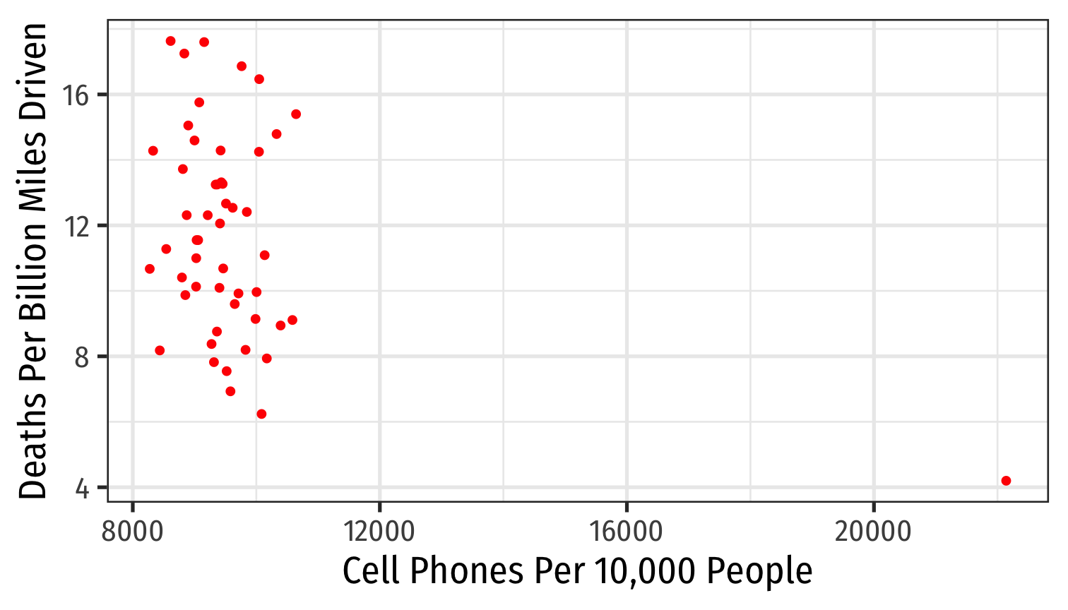
- Time-series data: track same individual ˉi over different times t
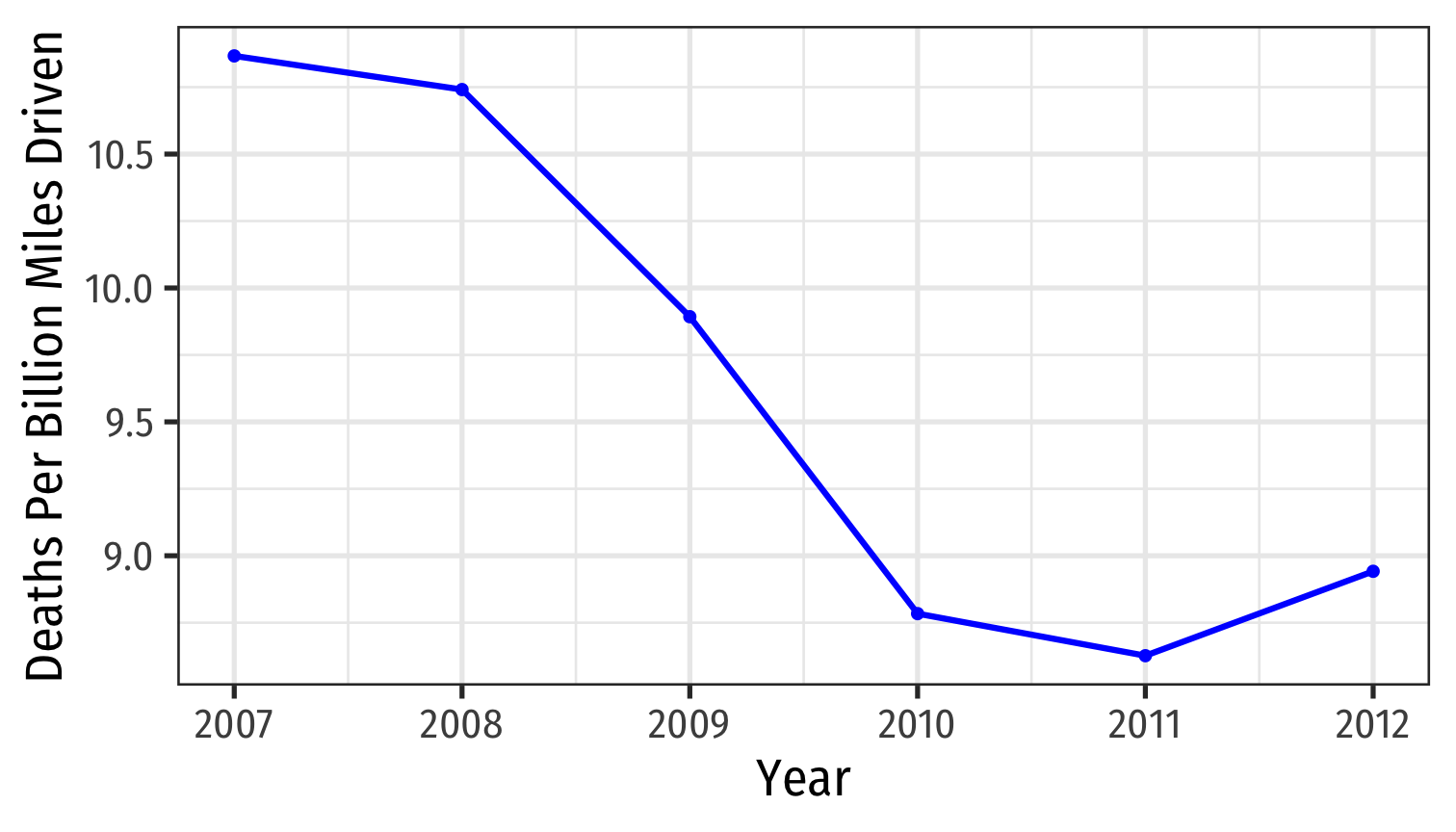
Types of Data I
- Cross-sectional data: compare different individual i’s at same time ˉt

- Time-series data: track same individual ˉi over different times t

- Panel data: combines these dimensions: compare all individual i’s over all time t’s
Panel Data I
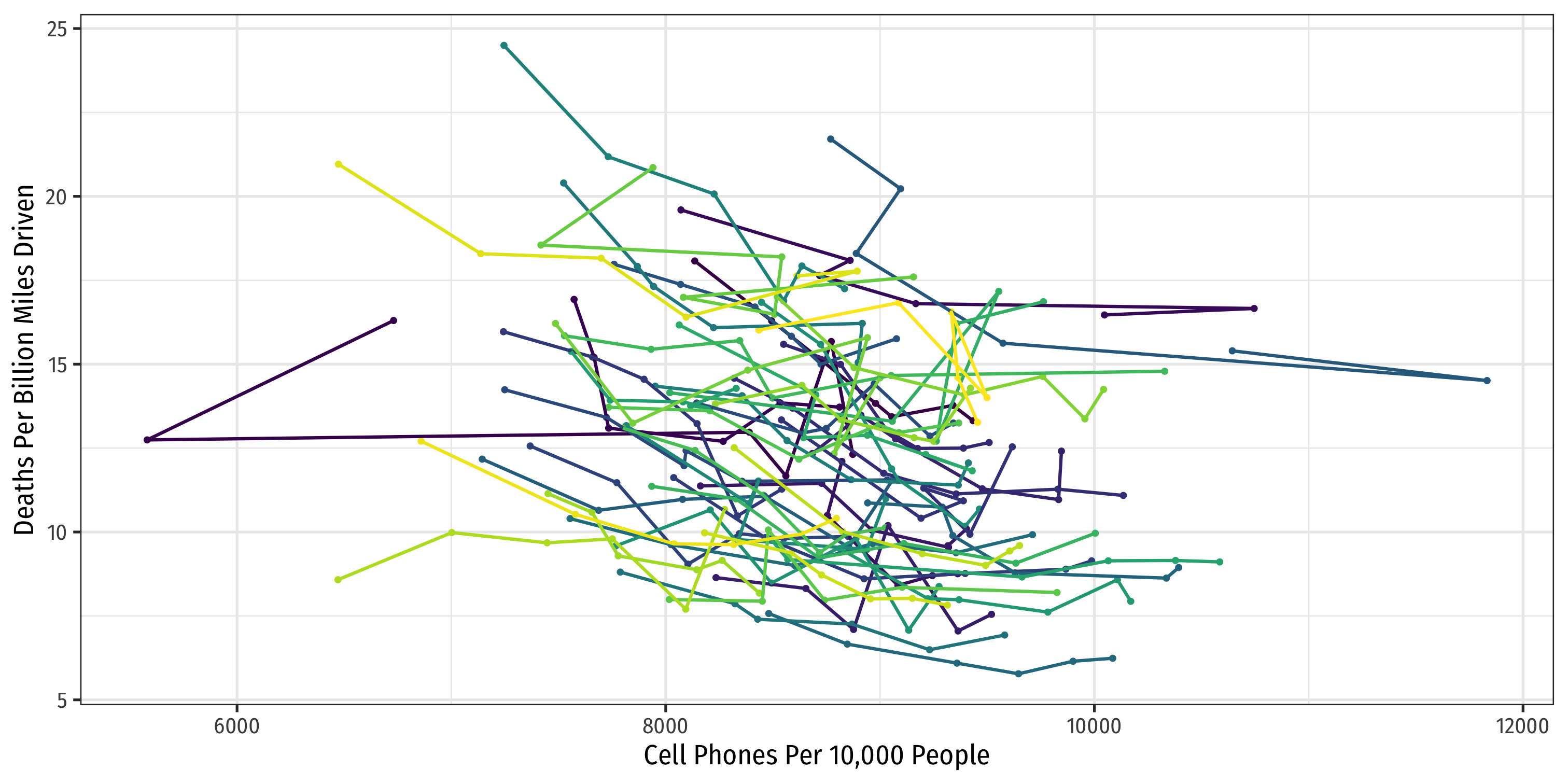
Panel Data II
| ABCDEFGHIJ0123456789 |
state <fctr> | year <fctr> | deaths <dbl> | |
|---|---|---|---|
| Alabama | 2007 | 18.075232 | |
| Alabama | 2008 | 16.289227 | |
| Alabama | 2009 | 13.833678 | |
| Alabama | 2010 | 13.434084 | |
| Alabama | 2011 | 13.771989 | |
| Alabama | 2012 | 13.316056 | |
| Alaska | 2007 | 16.301184 | |
| Alaska | 2008 | 12.744090 | |
| Alaska | 2009 | 12.973849 | |
| Alaska | 2010 | 11.670893 |
- Panel or Longitudinal data contains
- repeated observations (t)
- on multiple individuals (i)
Panel Data II
| ABCDEFGHIJ0123456789 |
state <fctr> | year <fctr> | deaths <dbl> | |
|---|---|---|---|
| Alabama | 2007 | 18.075232 | |
| Alabama | 2008 | 16.289227 | |
| Alabama | 2009 | 13.833678 | |
| Alabama | 2010 | 13.434084 | |
| Alabama | 2011 | 13.771989 | |
| Alabama | 2012 | 13.316056 | |
| Alaska | 2007 | 16.301184 | |
| Alaska | 2008 | 12.744090 | |
| Alaska | 2009 | 12.973849 | |
| Alaska | 2010 | 11.670893 |
Panel or Longitudinal data contains
- repeated observations (t)
- on multiple individuals (i)
Thus, our regression equation looks like:
^Yit=β0+β1Xit+uit
for individual i in time t.
Panel Data: Our Motivating Example
| ABCDEFGHIJ0123456789 |
state <fctr> | year <fctr> | deaths <dbl> | |
|---|---|---|---|
| Alabama | 2007 | 18.075232 | |
| Alabama | 2008 | 16.289227 | |
| Alabama | 2009 | 13.833678 | |
| Alabama | 2010 | 13.434084 | |
| Alabama | 2011 | 13.771989 | |
| Alabama | 2012 | 13.316056 | |
| Alaska | 2007 | 16.301184 | |
| Alaska | 2008 | 12.744090 | |
| Alaska | 2009 | 12.973849 | |
| Alaska | 2010 | 11.670893 |
Example: Do cell phones cause more traffic fatalities?
No measure of cell phones used while driving
cell_plansas a proxy for cell phone usage
State-level data over 6 years
The Data I
glimpse(phones)## Rows: 306## Columns: 8## $ year <fct> 2007, 2007, 2007, 2007, 2007, 2007, 2007, 2007, 2007, 2…## $ state <fct> Alabama, Alaska, Arizona, Arkansas, California, Colorad…## $ urban_percent <dbl> 30, 55, 45, 21, 54, 34, 84, 31, 100, 53, 39, 45, 11, 56…## $ cell_plans <dbl> 8135.525, 6730.282, 7572.465, 8071.125, 8821.933, 8162.…## $ cell_ban <fct> 0, 0, 0, 0, 0, 0, 1, 0, 1, 0, 0, 0, 0, 0, 0, 0, 0, 0, 0…## $ text_ban <fct> 0, 0, 0, 0, 0, 0, 1, 0, 1, 0, 0, 0, 0, 0, 0, 0, 0, 0, 0…## $ deaths <dbl> 18.075232, 16.301184, 16.930578, 19.595430, 12.104340, …## $ year_num <dbl> 2007, 2007, 2007, 2007, 2007, 2007, 2007, 2007, 2007, 2…The Data II
phones %>% count(year)| ABCDEFGHIJ0123456789 |
year <fctr> | n <int> | |||
|---|---|---|---|---|
| 2007 | 51 | |||
| 2008 | 51 | |||
| 2009 | 51 | |||
| 2010 | 51 | |||
| 2011 | 51 | |||
| 2012 | 51 |
The Data IV
phones %>% summarize(States = n_distinct(state), Years = n_distinct(year))| ABCDEFGHIJ0123456789 |
States <int> | Years <int> | |||
|---|---|---|---|---|
| 51 | 6 |
The Data: With plm
# install.packages("plm")library(plm)pdim(phones, index=c("state","year"))## Balanced Panel: n = 51, T = 6, N = 306plmpackage for panel data in Rpdim()checks dimensions of panel datasetindex=vector of "group" & "year" variables
Returns with a summary of:
ngroupsTperiodsNtotal observaitons
Pooled Regression I
- What if we just ran a standard regression:
^Yit=β0+β1Xit+uit
Pooled Regression I
- What if we just ran a standard regression:
^Yit=β0+β1Xit+uit
- N number of i groups (e.g. U.S. States)
- T number of t periods (e.g. years)
- This is a pooled regression model: treats all observations as independent
Pooled Regression II
pooled <- lm(deaths ~ cell_plans, data = phones)pooled %>% tidy()| ABCDEFGHIJ0123456789 |
term <chr> | estimate <dbl> | std.error <dbl> | statistic <dbl> | p.value <dbl> |
|---|---|---|---|---|
| (Intercept) | 17.3371034167 | 0.975384504 | 17.774635 | 5.821724e-49 |
| cell_plans | -0.0005666385 | 0.000106975 | -5.296926 | 2.264086e-07 |
Pooled Regression III
ggplot(data = phones)+ aes(x = cell_plans, y = deaths)+ geom_point()+ labs(x = "Cell Phones Per 10,000 People", y = "Deaths Per Billion Miles Driven")+ theme_bw(base_family = "Fira Sans Condensed", base_size=14)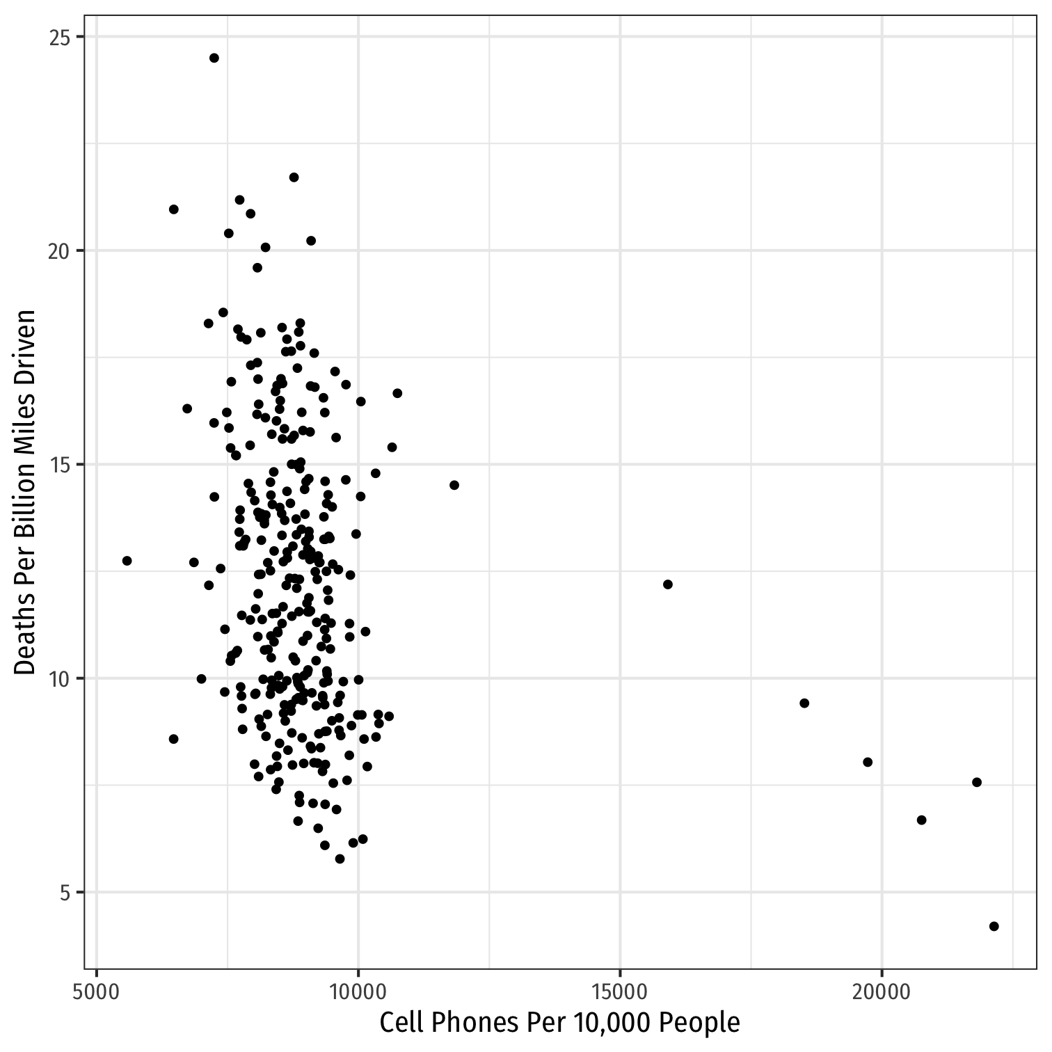
Pooled Regression III
ggplot(data = phones)+ aes(x = cell_plans, y = deaths)+ geom_point()+ geom_smooth(method = "lm", color = "red")+ labs(x = "Cell Phones Per 10,000 People", y = "Deaths Per Billion Miles Driven")+ theme_bw(base_family = "Fira Sans Condensed", base_size=14)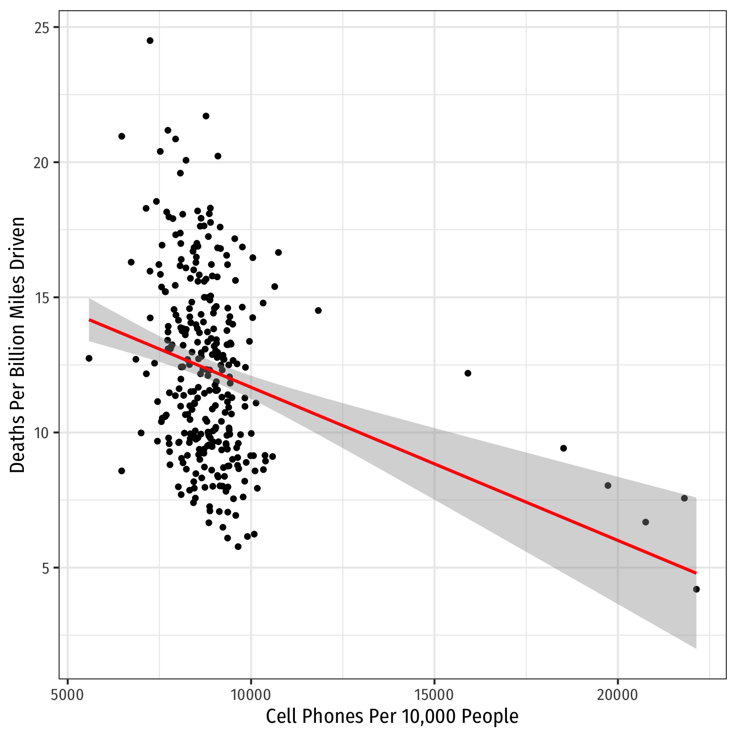
Recap: Assumptions about Errors
- Recall the 4 critical assumptions about u:
The expected value of the residuals is 0 E[u]=0
The variance of the residuals over X is constant: var(u|X)=σ2u
Errors are not correlated across observations: cor(ui,uj)=0∀i≠j
There is no correlation between X and the error term: cor(X,u)=0 or E[u|X]=0

Biases of Pooled Regression
^Yit=β0+β1Xit+ϵit
Assumption 3: cor(ui,uj)=0∀i≠j
Pooled regression model is biased because it ignores:
- Multiple observations from same group i
- Multiple observations from same time t
Thus, errors are serially or auto-correlated; cor(ui,uj)≠0 within same i and within same t
Biases of Pooled Regression: Our Example
^Deathsit=β0+β1Cell Phonesit+uit
Multiple observations from same state i
- Probably similarities among u for obs in same state
- Residuals on observations from same state are likely correlated
Multiple observations from same year t
- Probably similarities among u for obs in same year
- Residuals on observations from same year are likely correlated
Example: Consider Just 5 States
phones %>% filter(state %in% c("District of Columbia", "Maryland", "Texas", "California", "Kansas")) %>%ggplot(data = .)+ aes(x = cell_plans, y = deaths, color = state)+ geom_point()+ geom_smooth(method = "lm")+ labs(x = "Cell Phones Per 10,000 People", y = "Deaths Per Billion Miles Driven", color = NULL)+ theme_bw(base_family = "Fira Sans Condensed", base_size=14)+ theme(legend.position = "top")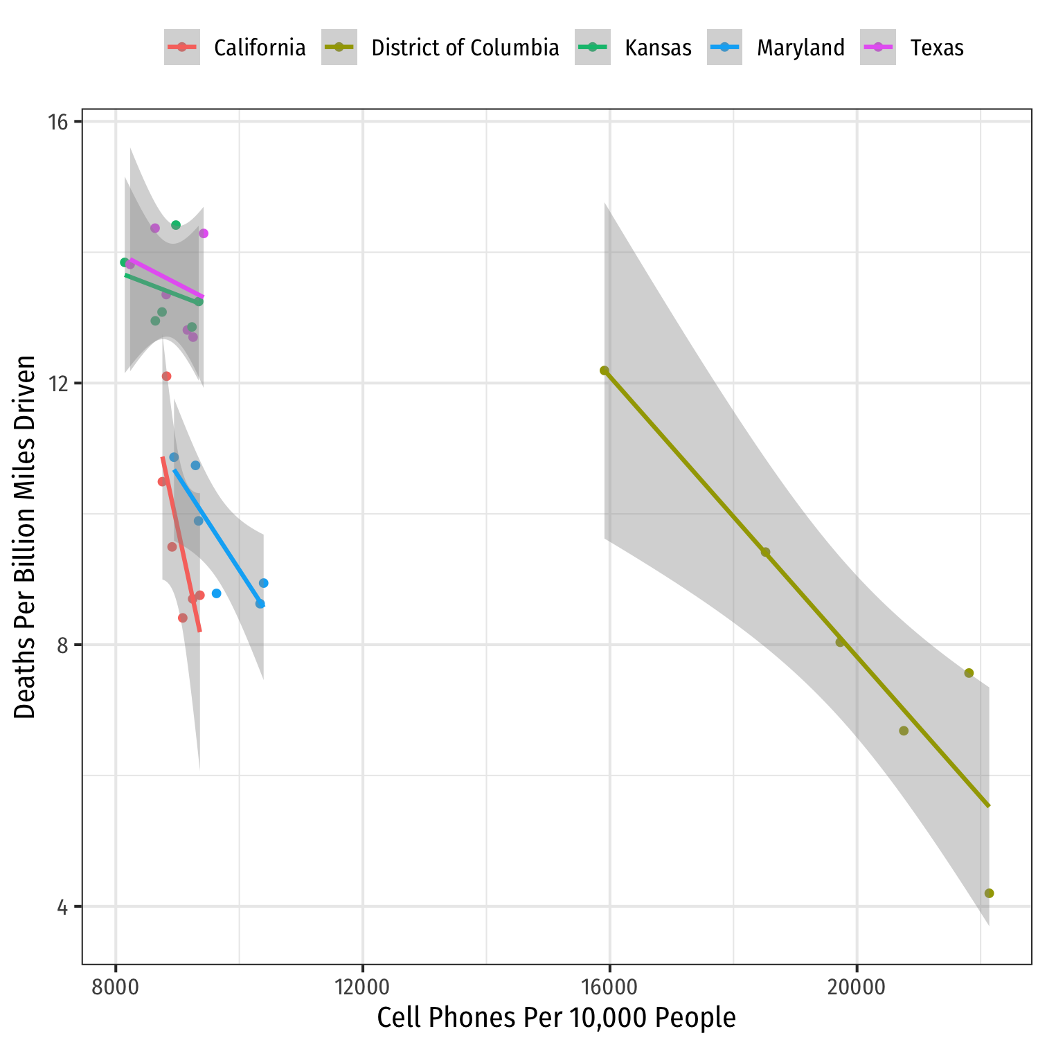
Example: Consider Just 5 States
phones %>% filter(state %in% c("District of Columbia", "Maryland", "Texas", "California", "Kansas")) %>%ggplot(data = .)+ aes(x = cell_plans, y = deaths, color = state)+ geom_point()+ geom_smooth(method = "lm")+ labs(x = "Cell Phones Per 10,000 People", y = "Deaths Per Billion Miles Driven", color = NULL)+ theme_bw(base_family = "Fira Sans Condensed", base_size=14)+ theme(legend.position = "none")+ facet_wrap(~state, ncol=3)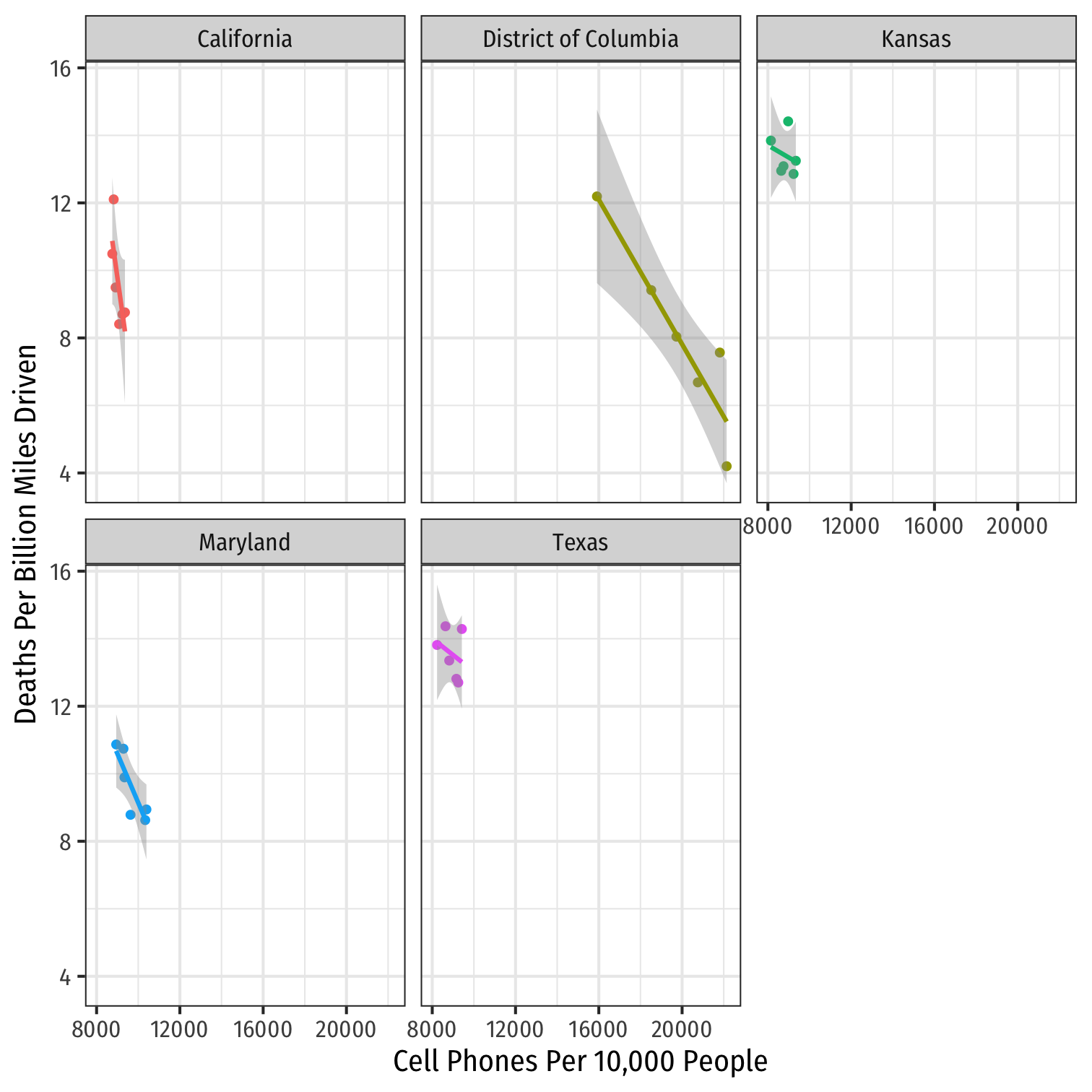
Look at All States
ggplot(data = phones)+ aes(x = cell_plans, y = deaths, color = state)+ geom_point()+ geom_smooth(method = "lm")+ labs(x = "Cell Phones Per 10,000 People", y = "Deaths Per Billion Miles Driven", color = NULL)+ theme_bw(base_family = "Fira Sans Condensed")+ theme(legend.position = "none")+ facet_wrap(~state, ncol=7)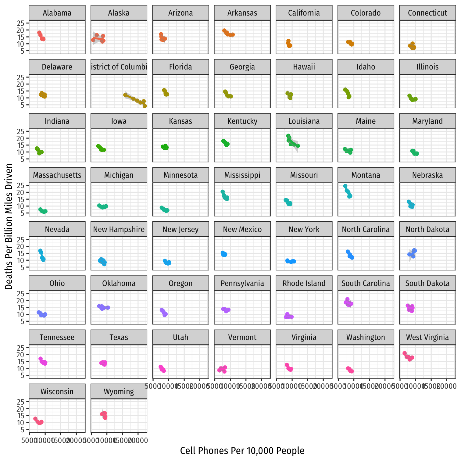
The Bias in our Pooled Regression
^Deathsit=β0+β1Cell Phonesit+uit
- Cell Phonesit is endogenous:
The Bias in our Pooled Regression
^Deathsit=β0+β1Cell Phonesit+uit
- Cell Phonesit is endogenous:
cor(uit,cell phonesit)≠0E[uit|cell phonesit]≠0
The Bias in our Pooled Regression
^Deathsit=β0+β1Cell Phonesit+uit
- Cell Phonesit is endogenous:
cor(uit,cell phonesit)≠0E[uit|cell phonesit]≠0
- Things in uit correlated with Cell phonesit:
- infrastructure spending, population, urban vs. rural, more/less cautious citizens, cultural attitudes towards driving, texting, etc
- A lot of these things vary systematically by State!
- cor(uit1,uit2)≠0
- Error in State i during t1 correlates with error in State i during t2
- things in State that don’t change over time
- cor(uit1,uit2)≠0
Fixed Effects Model
Fixed Effects: DAG
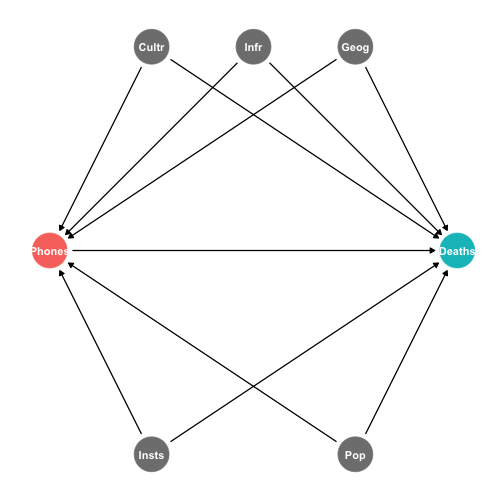
A simple pooled model likely contains lots of omitted variable bias
Many (often unobservable) factors that determine both Phones & Deaths
- Culture, infrastructure, population, geography, institutions, etc
Fixed Effects: DAG
A simple pooled model likely contains lots of omitted variable bias
Many (often unobservable) factors that determine both Phones & Deaths
- Culture, infrastructure, population, geography, institutions, etc
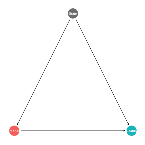
But the beauty of this is that most of these factors systematically vary by U.S. State and are stable over time!
We can simply “control for State” to safely remove the influence of all of these factors!
Fixed Effects: Decomposing uit
- Much of the endogeneity in Xit can be explained by systematic differences across i (groups)
Fixed Effects: Decomposing uit
Much of the endogeneity in Xit can be explained by systematic differences across i (groups)
Exploit the systematic variation across groups with a fixed effects model
Fixed Effects: Decomposing uit
Much of the endogeneity in Xit can be explained by systematic differences across i (groups)
Exploit the systematic variation across groups with a fixed effects model
Decompose the model error term into two parts:
uit=αi+ϵit
Fixed Effects: αi
- Decompose the model error term into two parts:
uit=αi+ϵit
αi are group-specific fixed effects
- group i tends to have higher or lower ˆY than other groups given regressor(s) Xit
- estimate a separate αi for each group i
- essentially, estimate a separate constant (intercept) for each group
- notice this is stable over time within each group (subscript only i, no t)
This includes all factors that do not change within group i over time
Fixed Effects: ϵit
uit=αi+ϵit
ϵit is the remaining random error
- As usual in OLS, assume the 4 typical assumptions about this error:
- E[ϵit]=0, var[ϵit]=σ2ϵ, cor(ϵit,ϵjt)=0, cor(ϵit,Xit)=0
ϵit includes all other factors affecting Yit not contained in group effect αi
- i.e. differences within each group that change over time
- Be careful: Xit can still be endogenous from other factors!
Fixed Effects: New Regression Equation
ˆYit=β0+β1Xit+αi+ϵit
We've pulled αi out of the original error term into the regression
Essentially we’ll estimate an intercept for each group (minus one, which is β0)
- avoiding the dummy variable trap
Must have multiple observations (over time) for each group (i.e. panel data)
Fixed Effects: Our Example
^Deathsit=β0+β1Cell phonesit+αi+ϵit
αi is the State fixed effect
- Captures everything unique about each state i that does not change over time
- culture, institutions, history, geography, climate, etc!
There could still be factors in ϵit that are correlated with Cell phonesit!
- things that do change over time within States
- perhaps individual States have cell phone bans for some years in our data
Estimating Fixed Effects Models
ˆYit=β0+β1Xit+αi+ϵit
- Two methods to estimate fixed effects models:
Least Squares Dummy Variable (LSDV) approach
De-meaned data approach
Least Squares Dummy Variable Approach
Least Squares Dummy Variable Approach
^Yit=β0+β1Xit+β2D1i+β3D2i+⋯+βND(N−1)i+ϵit
- A dummy variable Di={0,1} for each possible group
- =1 if observation it is from group i, otherwise =0
Least Squares Dummy Variable Approach
^Yit=β0+β1Xit+β2D1i+β3D2i+⋯+βND(N−1)i+ϵit
- A dummy variable Di={0,1} for each possible group
- =1 if observation it is from group i, otherwise =0
- If there are N groups:
- Include N−1 dummies (to avoid dummy variable trap) and β0 is the reference category†
- So we are estimating a different intercept for each group
- Sounds like a lot of work, automatic in
R
Least Squares Dummy Variable Approach: Our Example
Example: ^Deathsit=β0+β1Cell Phonesit+Alaskai+⋯+Wyomingi
- Let Alabama be the reference category (β0), include all other States
Our Example in R I
^Deathsit=β0+β1Cell Phonesit+Alaskai+⋯+Wyomingi
If
stateis afactorvariable, just include it in the regressionRautomatically creates N−1 dummy variables and includes them in the regression- Keeps intercept and leaves out first group dummy
Our Example in R II
fe_reg_1 <- lm(deaths ~ cell_plans + state, data = phones)fe_reg_1 %>% tidy()| ABCDEFGHIJ0123456789 |
term <chr> | estimate <dbl> | std.error <dbl> | statistic <dbl> | p.value <dbl> |
|---|---|---|---|---|
| (Intercept) | 25.507679925 | 1.0176400289 | 25.06552337 | 1.241581e-70 |
| cell_plans | -0.001203742 | 0.0001013125 | -11.88147584 | 3.483442e-26 |
| stateAlaska | -2.484164783 | 0.6745076282 | -3.68293060 | 2.816972e-04 |
| stateArizona | -1.510577383 | 0.6704569688 | -2.25305643 | 2.510925e-02 |
| stateArkansas | 3.192662931 | 0.6664383936 | 4.79063476 | 2.829319e-06 |
| stateCalifornia | -4.978668651 | 0.6655467951 | -7.48056889 | 1.206933e-12 |
| stateColorado | -4.344553493 | 0.6654735335 | -6.52851432 | 3.588784e-10 |
| stateConnecticut | -6.595185530 | 0.6654428902 | -9.91097152 | 8.698802e-20 |
| stateDelaware | -2.098393628 | 0.6666483193 | -3.14767707 | 1.842218e-03 |
| stateDistrict of Columbia | 6.355790010 | 1.2897172620 | 4.92804911 | 1.499627e-06 |
De-meaned Approach
De-meaned Approach I
Alternatively, we can control our regression for group fixed effects without directly estimating them
We simply de-mean the data for each group
De-meaned Approach I
Alternatively, we can control our regression for group fixed effects without directly estimating them
We simply de-mean the data for each group
For each group i, find the means (over time, t): ˉYi=β0+β1ˉXi+ˉαi+ˉϵit
De-meaned Approach I
Alternatively, we can control our regression for group fixed effects without directly estimating them
We simply de-mean the data for each group
For each group i, find the means (over time, t): ˉYi=β0+β1ˉXi+ˉαi+ˉϵit
- Where:
- ˉYi: average value of Yit for group i
- ˉXi: average value of Xit for group i
- ˉαi: average value of αi for group i (=αi)
- ˉϵit=0, by assumption 1
De-meaned Approach II
^Yit=β0+β1Xit+uitˉYi=β0+β1ˉXi+ˉαi+ˉϵi
De-meaned Approach II
^Yit=β0+β1Xit+uitˉYi=β0+β1ˉXi+ˉαi+ˉϵi
- Subtract the means equation from the pooled equation to get:
Yi−ˉYi=β1(Xit−ˉXi)+˜ϵit˜Yit=β1˜Xit+˜ϵit
De-meaned Approach II
^Yit=β0+β1Xit+uitˉYi=β0+β1ˉXi+ˉαi+ˉϵi
- Subtract the means equation from the pooled equation to get:
Yi−ˉYi=β1(Xit−ˉXi)+˜ϵit˜Yit=β1˜Xit+˜ϵit
Within each group i, the de-meaned variables ˜Yit and ˜Xit's all have a mean of 0†
Variables that don't change over time will drop out of analysis altogether
Removes any source of variation across groups to only work with variation within each group
† Recall Rule 4 from the 2.3 class notes on the Summation Operator: ∑(Xi−ˉX)=0
De-meaned Approach III
˜Yit=β1˜Xit+˜ϵit
Yields identical results to dummy variable approach
More useful when we have many groups (would be many dummies)
Demonstrates intuition behind fixed effects:
- Converts all data to deviations from the mean of each group
- All groups are “centered” at 0
- Fixed effects are often called the “within” estimators, they exploit variation within groups, not across groups
De-meaned Approach IV
We are basically comparing groups to themselves over time
- apples to apples comparison
- e.g. Maryland in 2000 vs. Maryland in 2005
Ignore all differences between groups, only look at differences within groups over time
De-Meaning the Data in R I
# get means of Y and X by statemeans_state<-phones %>% group_by(state) %>% summarize(avg_deaths = mean(deaths), avg_phones = mean(cell_plans))# look at itmeans_stateDe-Meaning the Data in R I
# get means of Y and X by statemeans_state<-phones %>% group_by(state) %>% summarize(avg_deaths = mean(deaths), avg_phones = mean(cell_plans))# look at itmeans_state| ABCDEFGHIJ0123456789 |
state <fctr> | avg_deaths <dbl> | avg_phones <dbl> |
|---|---|---|
| Alabama | 14.786711 | 8906.370 |
| Alaska | 13.612953 | 7817.759 |
| Arizona | 14.249825 | 8097.482 |
| Arkansas | 17.543881 | 9268.153 |
| California | 9.659712 | 9029.594 |
| Colorado | 10.351405 | 8981.762 |
| Connecticut | 8.141739 | 8947.729 |
| Delaware | 12.209610 | 9304.052 |
| District of Columbia | 8.015895 | 19811.205 |
| Florida | 13.544635 | 9078.592 |
De-Meaning the Data in R II
ggplot(data = means_state)+ aes(x = fct_reorder(state, avg_deaths), y = avg_deaths, color = state)+ geom_point()+ geom_segment(aes(y = 0, yend = avg_deaths, x = state, xend = state))+ coord_flip()+ labs(x = "Cell Phones Per 10,000 People", y = "Deaths Per Billion Miles Driven", color = NULL)+ theme_bw(base_family = "Fira Sans Condensed", base_size=10)+ theme(legend.position = "none")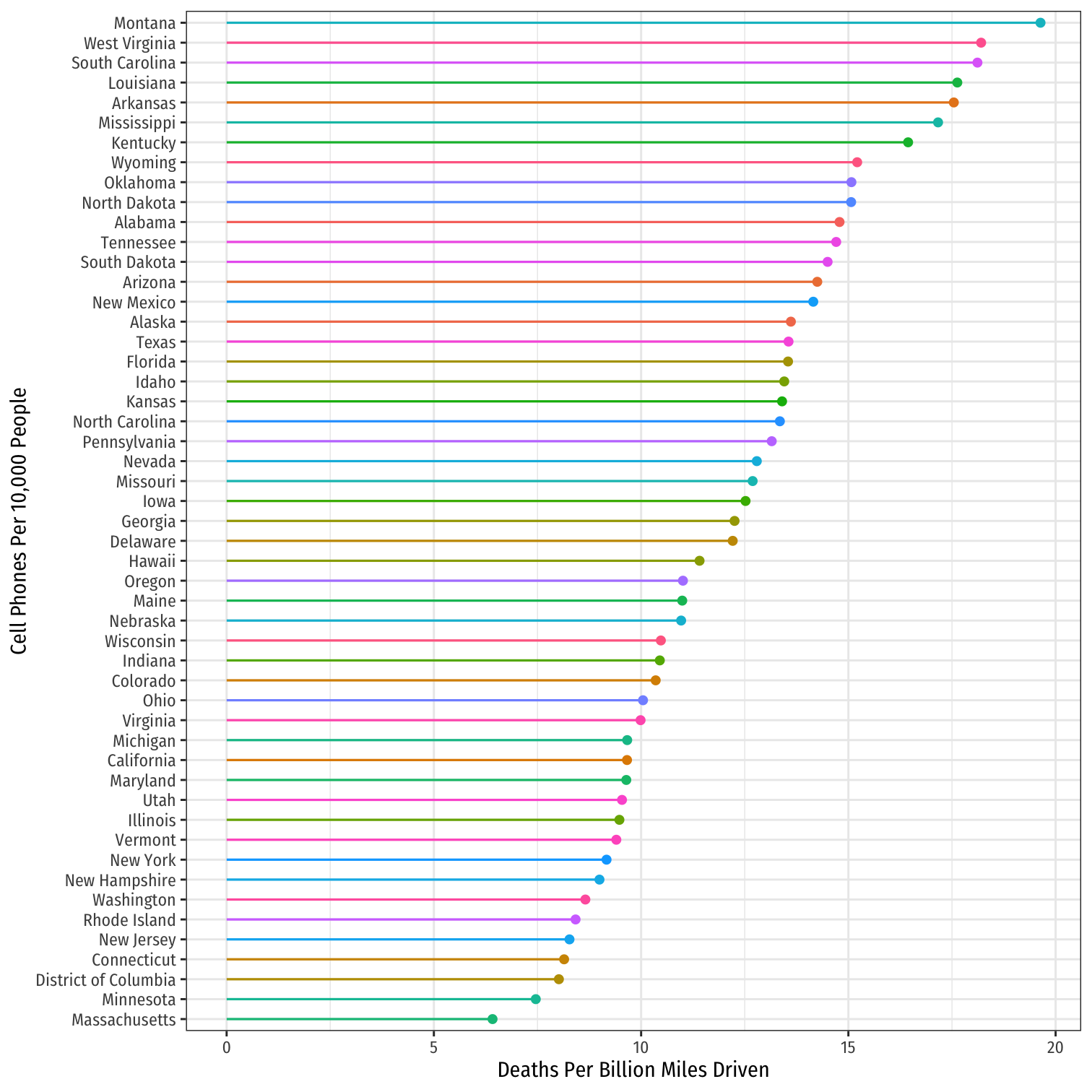
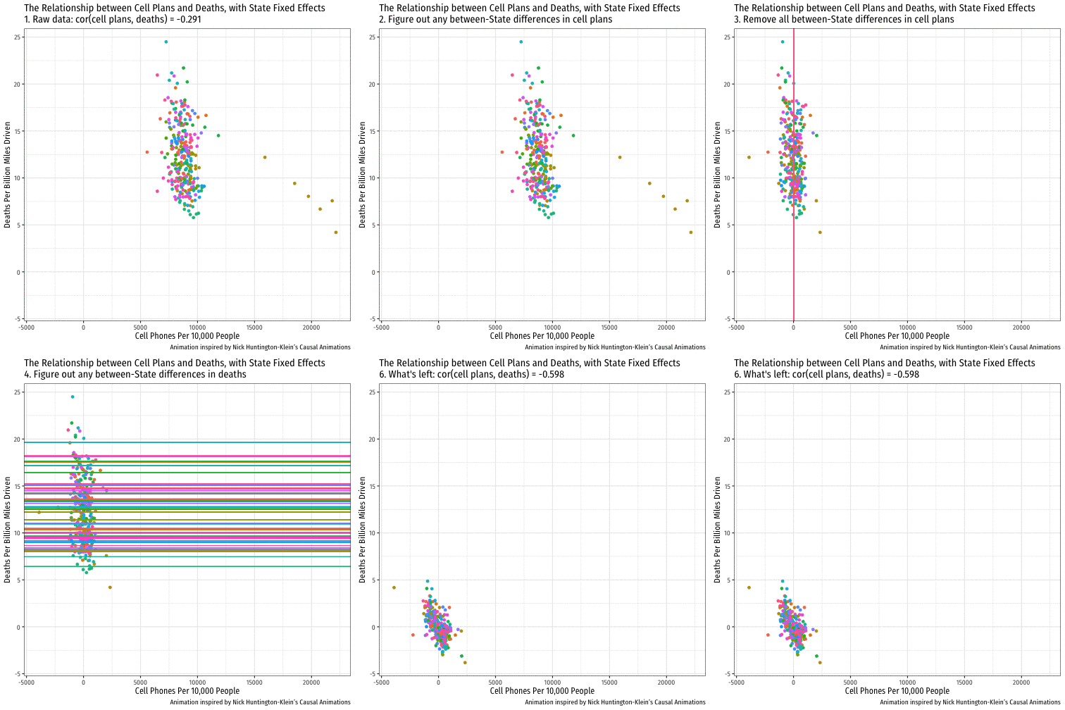
Visualizing "Within Estimates" for the 5 States
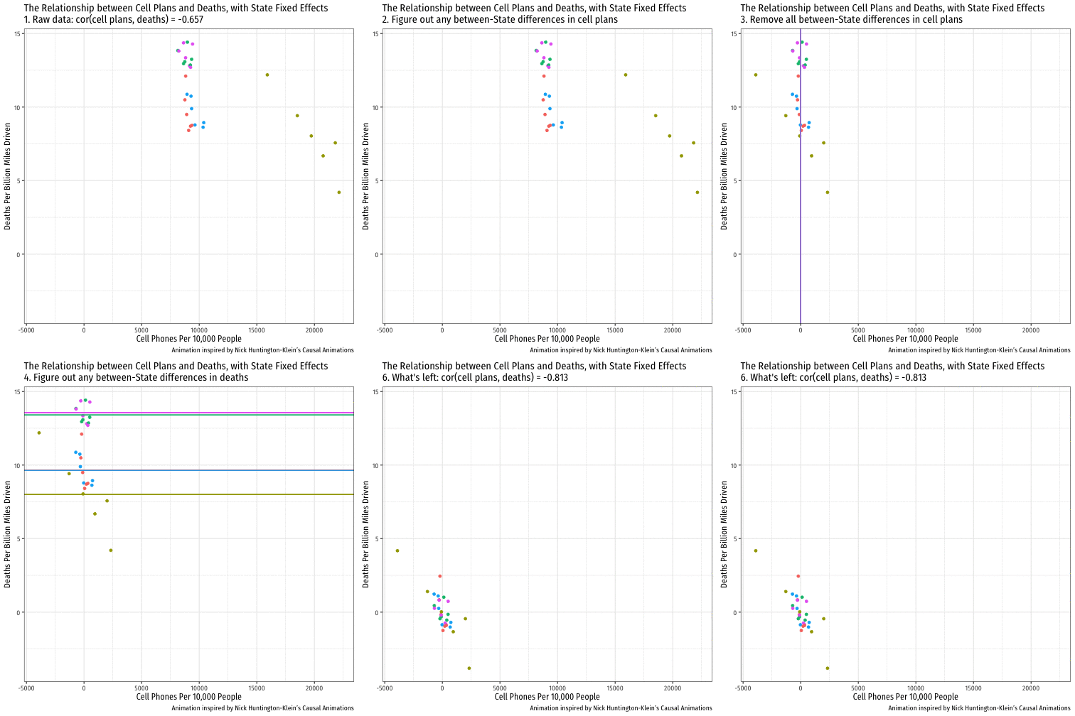
Visualizing "Within Estimates" for All 51 States
De-meaned Approach in R I
The
plmpackage is designed for panel dataplm()function is just likelm(), with some additional arguments:index="group_variable_name"set equal to the name of yourfactorvariable for the groupsmodel=set equal to"within"to use fixed-effects (within-estimator)
#install.packages("plm")library(plm)fe_reg_1_alt<-plm(deaths ~ cell_plans, data = phones, index = "state", model = "within")De-meaned Approach in R II
fe_reg_1_alt %>% tidy()| ABCDEFGHIJ0123456789 |
term <chr> | estimate <dbl> | std.error <dbl> | statistic <dbl> | p.value <dbl> |
|---|---|---|---|---|
| cell_plans | -0.001203742 | 0.0001013125 | -11.88148 | 3.483442e-26 |
Two-Way Fixed Effects
Two-Way Fixed Effects
State fixed effect controls for all factors that vary by state but are stable over time
But there are still other (often unobservable) factors that affect both Phones and Deaths, that don’t vary by State
- The country’s macroeconomic performance, federal laws, etc
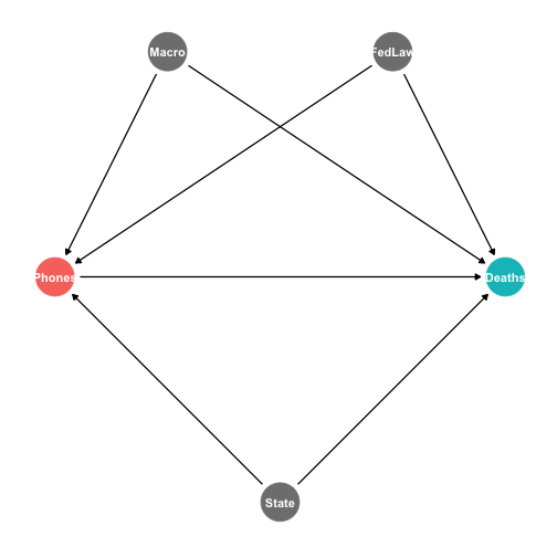
Two-Way Fixed Effects
State fixed effect controls for all factors that vary by state but are stable over time
But there are still other (often unobservable) factors that affect both Phones and Deaths, that don’t vary by State
- The country’s macroeconomic performance, federal laws, etc
If these factors systematically vary over time, but are the same by State, then we can “control for Year” to safely remove the influence of all of these factors!
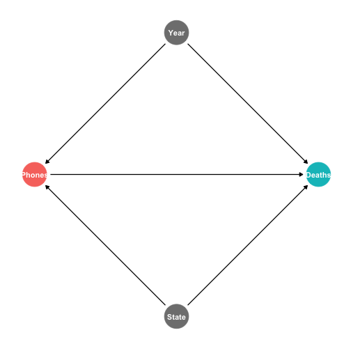
Two-Way Fixed Effects
- A one-way fixed effects model estimates a fixed effect for groups
Two-Way Fixed Effects
A one-way fixed effects model estimates a fixed effect for groups
Two-way fixed effects model estimates fixed effects for both groups and time periods ^Yit=β0+β1Xit+αi+θt+νit
αi: group fixed effects
- accounts for time-invariant differences across groups
θt: time fixed effects
- accounts for group-invariant differences over time
νit remaining random error
- all remaining factors that affect Yit that vary by state and change over time
Two-Way Fixed Effects: Our Example
^Deathsit=β0+β1Cell phonesit+αi+θt+νit
αi: State fixed effects
- differences across states that are stable over time (note subscript i only)
- e.g. geography, culture, (unchanging) state laws
θt: Year fixed effects
- differences over time that are stable across states (note subscript t only)
- e.g. economy-wide macroeconomic changes, federal laws passed
Visualizing Year Effects I
# find averages for yearsmeans_year<-phones %>% group_by(year) %>% summarize(avg_deaths = mean(deaths), avg_phones = mean(cell_plans))means_year| ABCDEFGHIJ0123456789 |
year <fctr> | avg_deaths <dbl> | avg_phones <dbl> | ||
|---|---|---|---|---|
| 2007 | 14.00751 | 8064.531 | ||
| 2008 | 12.87156 | 8482.903 | ||
| 2009 | 12.08632 | 8859.706 | ||
| 2010 | 11.61487 | 9134.592 | ||
| 2011 | 11.36431 | 9485.238 | ||
| 2012 | 11.65666 | 9660.474 |
Visualizing Year Effects II
ggplot(data = phones)+ aes(x = year, y = deaths)+ geom_point(aes(color = year))+ # Add the yearly means as black points geom_point(data = means_year, aes(x = year, y = avg_deaths), size = 3, color = "black")+ geom_path(data = means_year, aes(x = year, y = avg_deaths), size = 1)+ theme_bw(base_family = "Fira Sans Condensed", base_size = 14)+ theme(legend.position = "none")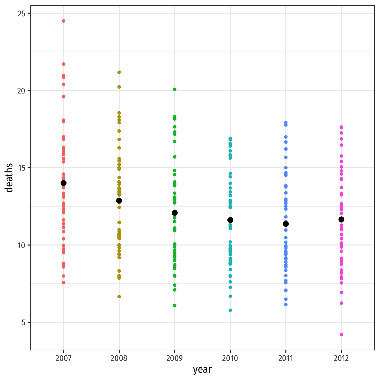
Estimating Two-Way Fixed Effects
ˆYit=β0+β1Xit+αi+θt+νit
- As before, several equivalent ways to estimate two-way fixed effects models:
1) Least Squares Dummy Variable (LSDV) Approach: add dummies for both groups and time periods (separate intercepts for groups and times)
Estimating Two-Way Fixed Effects
ˆYit=β0+β1Xit+αi+θt+νit
- As before, several equivalent ways to estimate two-way fixed effects models:
1) Least Squares Dummy Variable (LSDV) Approach: add dummies for both groups and time periods (separate intercepts for groups and times)
2) Fully De-meaned data: ˜Yit=β1˜Xit+˜νit
where for each variable: ~varit=varit−¯vart−¯vari
3) Hybrid: de-mean for one effect (groups or years) and add dummies for the other effect (years or groups)
LSDV Method
fe2_reg_1 <- lm(deaths ~ cell_plans + state + year, data = phones)fe2_reg_1 %>% tidy()| ABCDEFGHIJ0123456789 |
term <chr> | estimate <dbl> | std.error <dbl> | statistic <dbl> | p.value <dbl> |
|---|---|---|---|---|
| (Intercept) | 18.9304707399 | 1.4511323962 | 13.0453092 | 5.427406e-30 |
| cell_plans | -0.0002995294 | 0.0001723149 | -1.7382677 | 8.339982e-02 |
| stateAlaska | -1.4998292482 | 0.6241082951 | -2.4031554 | 1.698648e-02 |
| stateArizona | -0.7791714713 | 0.6113519094 | -1.2745057 | 2.036724e-01 |
| stateArkansas | 2.8655344756 | 0.5985062952 | 4.7878101 | 2.895040e-06 |
| stateCalifornia | -5.0900897113 | 0.5956293282 | -8.5457338 | 1.299236e-15 |
| stateColorado | -4.4127241692 | 0.5953924847 | -7.4114543 | 1.945083e-12 |
| stateConnecticut | -6.6325834801 | 0.5952933996 | -11.1417051 | 1.169797e-23 |
| stateDelaware | -2.4579829953 | 0.5991822226 | -4.1022295 | 5.546475e-05 |
| stateDistrict of Columbia | -3.5044963616 | 1.9710939218 | -1.7779449 | 7.663326e-02 |
With plm
fe2_reg_2 <- plm(deaths ~ cell_plans, index = c("state", "year"), model = "within", data = phones)fe2_reg_2 %>% tidy()| ABCDEFGHIJ0123456789 |
term <chr> | estimate <dbl> | std.error <dbl> | statistic <dbl> | p.value <dbl> |
|---|---|---|---|---|
| cell_plans | -0.001203742 | 0.0001013125 | -11.88148 | 3.483442e-26 |
plm()command allows for multiple effects to be fit insideindex=c("group", "time")
Adding Covariates
State fixed effect absorbs all unobserved factors that vary by state, but are constant over time
Year fixed effect absorbs all unobserved factors that vary by year, but are constant over States
But there are still other (often unobservable) factors that affect both Phones and Deaths, that vary by State and change over time!
- Some States change their laws during the time period
- State urbanization rates change over the time period
We will also need to control for these variables (not picked up by fixed effects!)
- Add them to the regression
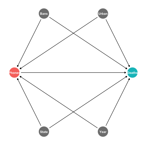
Adding Covariates I
^Deathsit=β1Cell Phonesit+αi+θt+urban pctit+cell banit+text banit
- Can still add covariates to remove endogeneity not soaked up by fixed effects
- factors that change within groups over time
- e.g. some states pass bans over the time period in data (some years before, some years after)
Adding Covariates II
fe2_controls_reg <- plm(deaths ~ cell_plans + text_ban + urban_percent + cell_ban, data = phones, index = c("state","year"), model = "within", effect = "twoways") fe2_controls_reg %>% tidy()| ABCDEFGHIJ0123456789 |
term <chr> | estimate <dbl> | std.error <dbl> | statistic <dbl> | p.value <dbl> |
|---|---|---|---|---|
| cell_plans | -0.0003403735 | 0.0001729402 | -1.968157 | 0.05017303 |
| text_ban1 | 0.2559261569 | 0.2221923049 | 1.151823 | 0.25051208 |
| urban_percent | 0.0131347657 | 0.0111986138 | 1.172892 | 0.24197354 |
| cell_ban1 | -0.6797956522 | 0.4029491232 | -1.687051 | 0.09286115 |
Comparing Models
library(huxtable)huxreg("Pooled" = pooled, "State Effects" = fe_reg_1, "State & Year Effects" = fe2_reg_1, "With Controls" = fe2_controls_reg, coefs = c("Intercept" = "(Intercept)", "Cell phones" = "cell_plans", "Cell Ban" = "cell_ban1", "Texting Ban" = "text_ban1", "Urbanization Rate" = "urban_percent"), statistics = c("N" = "nobs", "R-Squared" = "r.squared", "SER" = "sigma"), number_format = 4)| Pooled | State Effects | State & Year Effects | With Controls | |
|---|---|---|---|---|
| Intercept | 17.3371 *** | 25.5077 *** | 18.9305 *** | |
| (0.9754) | (1.0176) | (1.4511) | ||
| Cell phones | -0.0006 *** | -0.0012 *** | -0.0003 | -0.0003 |
| (0.0001) | (0.0001) | (0.0002) | (0.0002) | |
| Cell Ban | -0.6798 | |||
| (0.4029) | ||||
| Texting Ban | 0.2559 | |||
| (0.2222) | ||||
| Urbanization Rate | 0.0131 | |||
| (0.0112) | ||||
| N | 306 | 306 | 306 | 306 |
| R-Squared | 0.0845 | 0.9055 | 0.9259 | 0.0329 |
| SER | 3.2791 | 1.1526 | 1.0310 | |
| *** p < 0.001; ** p < 0.01; * p < 0.05. | ||||