3.6 — Regression with Categorical Data — Class Notes
Contents
Tuesday, October 27, 2020
Overview
Today we look at how to use data that is categorical (i.e. variables that indicate an observation’s membership in a particular group or category). We introduce them into regression models as dummy variables that can equal 0 or 1: where 1 indicates membership in a category, and 0 indicates non-membership.
We also look at what happens when categorical variables have more than two values: for regression, we introduce a dummy variable for each possible category - but be sure to leave out one reference category to avoid the dummy variable trap.
Readings
Please see today’s suggested readings.
Slides
Assignments
Problem Set 4 answers are posted on that page.
Live Class Session on Zoom
The live class Zoom meeting link can be found on Blackboard (see LIVE ZOOM MEETINGS on the left navigation menu), starting at 11:30 AM.
If you are unable to join today’s live session, or if you want to review, you can find the recording stored on Blackboard via Panopto (see Class Recordings on the left navigation menu).
Appendix: T-Test for Difference in Group Means
Often we want to compare the means between two groups, and see if the difference is statistically significant. As an example, is there a statistically significant difference in average hourly earnings between men and women? Let:
- \(\mu_W\): mean hourly earnings for female college graduates
- \(\mu_M\): mean hourly earnings for male college graduates
We want to run a hypothesis test for the difference \((d)\) in these two population means: \[\mu_M-\mu_W=d_0\]
Our null hypothesis is that there is no statistically significant difference. Let’s also have a two-sided alternative hypothesis, simply that there is a difference (positive or negative).
- \(H_0: d=0\)
- \(H_1: d \neq 0\)
Note a logical one-sided alternative would be \(H_2: d > 0\), i.e. men earn more than women
The Sampling Distribution of \(d\)
The true population means \(\mu_M, \mu_W\) are unknown, we must estimate them from samples of men and women. Let:
- \(\bar{Y}_M\) the average earnings of a sample of \(n_M\) men
- \(\bar{Y}_W\) the average earnings of a sample of \(n_W\) women
We then estimate \((\mu_M-\mu_W)\) with the sample \((\bar{Y}_M-\bar{Y}_W)\).
We would then run a t-test and calculate the test-statistic for the difference in means. The formula for the test statistic is:
\[t = \frac{(\bar{Y_M}-\bar{Y_W})-d_0}{\sqrt{\frac{s_M^2}{n_M}+\frac{s_W^2}{n_W}}}\]
We then compare \(t\) against the critical value \(t^*\), or calculate the \(p\)-value \(P(T>t)\) as usual to determine if we have sufficient evidence to reject \(H_0\)
## ── Attaching packages ─────────────────────────────────────── tidyverse 1.3.0 ──## ✓ ggplot2 3.3.2 ✓ purrr 0.3.4
## ✓ tibble 3.0.4 ✓ dplyr 1.0.2
## ✓ tidyr 1.1.2 ✓ stringr 1.4.0
## ✓ readr 1.3.1 ✓ forcats 0.5.0## ── Conflicts ────────────────────────────────────────── tidyverse_conflicts() ──
## x dplyr::filter() masks stats::filter()
## x dplyr::lag() masks stats::lag()library(wooldridge)
# Our data comes from wage1 in the wooldridge package
wages<-wooldridge::wage1
# look at average wage for men
wages %>%
filter(female==0) %>%
summarize(average = mean(wage),
sd = sd(wage))## average sd
## 1 7.099489 4.160858# look at average wage for women
wages %>%
filter(female==1) %>%
summarize(average = mean(wage),
sd = sd(wage))## average sd
## 1 4.587659 2.529363So our data is telling us that male and female average hourly earnings are distributed as such:
\[\begin{align*} \bar{Y}_M &\sim N(7.10,4.16)\\ \bar{Y}_W &\sim N(4.59,2.53)\\ \end{align*}\]
We can plot this to see visually. There is a lot of overlap in the two distributions, but the male average is higher than the female average, and there is also a lot more variation in males than females, noticeably the male distribution skews further to the right.
wages$female<-as.factor(wages$female)

library("ggplot2")
ggplot(data=wages,aes(x=wage,fill=female))+
  geom_density(alpha=0.5)+
  scale_x_continuous(seq(0,25,5),name="Wage",labels=scales::dollar)+
  theme_light()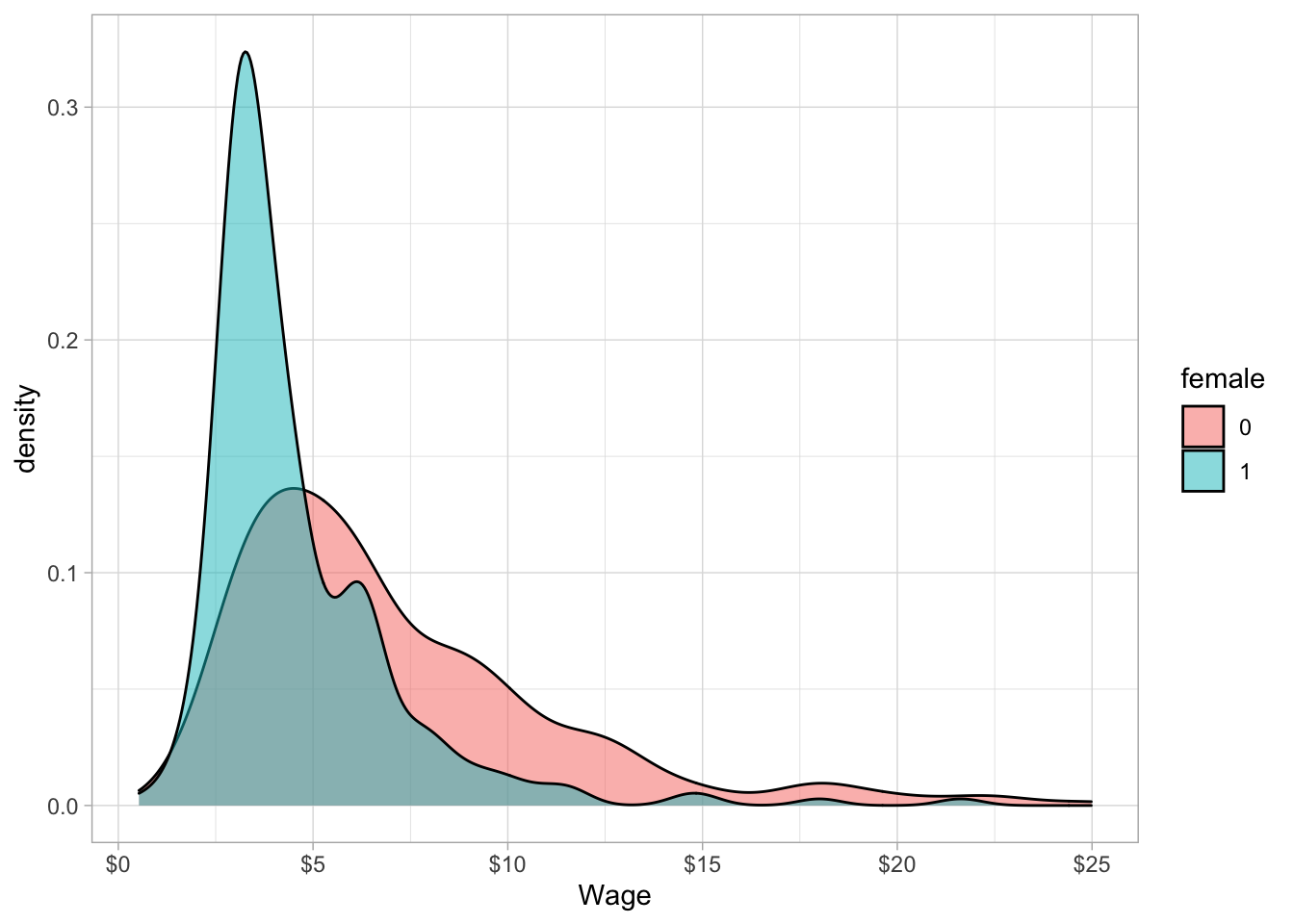
Knowing the distributions of male and female average hourly earnings, we can estimate the sampling distribution of the difference in group eans between men and women as:
The mean: \[\begin{align*} \bar{d}&=\bar{Y}_M-\bar{Y}_W\\ \bar{d}&=7.10-4.59\\ \bar{d}&=2.51\\ \end{align*}\]
The standard error of the mean: \[\begin{align*} SE(\bar{d})&=\sqrt{\frac{s_M^2}{n_M}+\frac{s_W^2}{n_W}}\\ &=\sqrt{\frac{4.16^2}{274}+\frac{2.33^2}{252}}\\ & \approx 0.29\\ \end{align*}\]
So the sampling distribution of the difference in group means is distributed: \[\bar{d} \sim N(2.51,0.29)\]
ggplot(data.frame(x=0:6),aes(x=x))+
  stat_function(fun=dnorm, args=list(mean=2.51, sd=0.29), color="purple")+
  ylab("Density")+
  scale_x_continuous(seq(0,6,1),name="Wage Difference",labels=scales::dollar)+
  theme_light()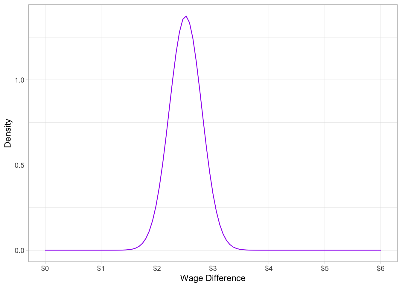
Now we the \(t\)-test like any other:
\[\begin{align*} t&=\frac{\text{estimate}-\text{null hypothesis}}{\text{standard error of the estimate}}\\ &=\frac{d-0}{SE(d)}\\ &=\frac{2.51-0}{0.29}\\ &=8.66\\ \end{align*}\]
This is statistically significant. The \(p\)-value, \(P(t>8.66)=\) is 0.000000000000000000410, or basically, 0.
## [1] 4.102729e-17The \(t\)-test in R
##
##  Welch Two Sample t-test
##
## data:  wage by female
## t = 8.44, df = 456.33, p-value = 4.243e-16
## alternative hypothesis: true difference in means is not equal to 0
## 95 percent confidence interval:
##  1.926971 3.096690
## sample estimates:
## mean in group 0 mean in group 1
## 7.099489 4.587659##
## Call:
## lm(formula = wage ~ female, data = wages)
##
## Residuals:
## Min 1Q Median 3Q Max
## -5.5995 -1.8495 -0.9877 1.4260 17.8805
##
## Coefficients:
## Estimate Std. Error t value Pr(>|t|)
## (Intercept) 7.0995 0.2100 33.806 < 2e-16 ***
## female1 -2.5118 0.3034 -8.279 1.04e-15 ***
## ---
## Signif. codes: 0 '***' 0.001 '**' 0.01 '*' 0.05 '.' 0.1 ' ' 1
##
## Residual standard error: 3.476 on 524 degrees of freedom
## Multiple R-squared: 0.1157, Adjusted R-squared: 0.114
## F-statistic: 68.54 on 1 and 524 DF, p-value: 1.042e-15