2.2 — Random Variables and Distributions — Class Notes
Contents
Tuesday, September 8, 2019
Overview
Today we finish your crash course/review of basic statistics with random variables and distributions.
Slides
Live Class Session on Zoom
The live class Zoom meeting link can be found on Blackboard (see LIVE ZOOM MEETINGS on the left navigation menu), starting at 11:30 AM.
If you are unable to join today’s live session, or if you want to review, you can find the recording stored on Blackboard via Panopto (see Class Recordings on the left navigation menu).
Problem Set
Problem Set 1 answers are posted on that page in various formats.
Problem set 2 (on classes 2.1-2.2) is posted shortly, and is will be due by Sunday September 13.
Math Appendix: Properties of Expected Value and Variance
There are several useful mathematical properties of expected value and variance.
Property 1: the expected value of a constant is itself, and the variance of a constant is 0.
\[\begin{align*} E(c)&=c\\ var(c)&=0\\ sd(c)&=0\\ \end{align*}\]
For any constant, \(c\)
- Example: \(E(2)=2\), \(var(2)=0\), \(sd(2)=0\)
Property 2: adding or subtracting a constant to a random variable and then taking the mean or variance:
\[\begin{align*} E(X \pm c)&=E(X) \pm c\\ var(X \pm c)&=X\\ sd(X \pm c)&=X\\ \end{align*}\]
For any constant, \(c\)
- Example: \(E(2+X)=2+E(X)\), \(var(2+X)=var(X)\), \(sd(2+X)=sd(X)\)
Property 3: multiplying a constant to a random variable and then taking the mean or variance:
\[\begin{align*} E(aX)&=E(X) aE(X)\\ var(aX)&=a^2var(X)\\ sd(aX)&=|a|sd(X)\\ \end{align*}\]
For any constant, \(a\)
- Example: \(E(2X)=2E(X)\), \(var(2X)=4var(X)\), \(sd(2X)=2sd(X)\)
Property 4: the expected value of the sum of two random variables is equal to the sum of each random variable’s expected value:
\[E(X \pm Y)=E(X) \pm E(Y)\]
R Appendix: Graphing Statistical and Mathematical Functions in R
The mosaic package is useful for making and using mathematical functions in R.
Creating Mathematical Functions
You can create custom mathematical functions using mosaic by defining an R function() with multiple arguments. As a simple example, make the function \(f(x) = 10x-x^2\) (with one argument, \(x\) since it is a univariate function) as follows:
# store as a named function, I'll call it "my_function"
my_function<-function(x){10*x-x^2}

# look at it
my_function
## function(x){10*x-x^2}There are some notational requirements from R for making functions. Any coefficient in front of a variable (such as the 10 in 10x must be explicitly multiplied by the variable, as in 10*x).
To use the function to calculate its value at a particular value of x, simply define what the (x) is and run your named function on it:
## [1] 16## [1] 16 24## [1] 16 21 24 25 24 21## [1] 16 24Graphing Mathematical Functions
In ggplot there is a dedicated stat_function() (equivalent to a geom_ layer) to graph mathematical and statistical functions. All that is needed is a data.frame of a range of x values to act as the source for data, and set x equal to those values for aesthetics.
## ── Attaching packages ─────────────────────────────────────── tidyverse 1.3.0 ──## ✓ tibble 3.0.4 ✓ purrr 0.3.4
## ✓ tidyr 1.1.2 ✓ stringr 1.4.0
## ✓ readr 1.3.1 ✓ forcats 0.5.0## ── Conflicts ────────────────────────────────────────── tidyverse_conflicts() ──
## x mosaic::count() masks dplyr::count()
## x purrr::cross() masks mosaic::cross()
## x mosaic::do() masks dplyr::do()
## x tidyr::expand() masks Matrix::expand()
## x dplyr::filter() masks stats::filter()
## x ggstance::geom_errorbarh() masks ggplot2::geom_errorbarh()
## x dplyr::lag() masks stats::lag()
## x tidyr::pack() masks Matrix::pack()
## x mosaic::stat() masks ggplot2::stat()
## x mosaic::tally() masks dplyr::tally()
## x tidyr::unpack() masks Matrix::unpack()
Then we add the stat_function, where fun = is the most important argument where you define the to function to graph as your function created above, for example, our my_function.
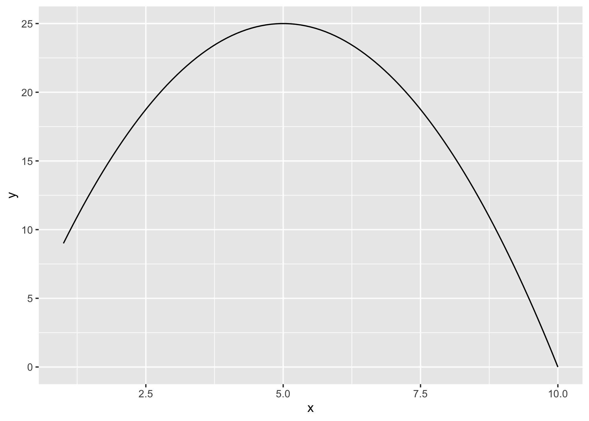
You can also adjust things like size, color, and line type.
ggplot(data = data.frame(x = 1:10))+
  aes(x = x)+
stat_function(fun = my_function, color = "blue", size = 2, linetype = "dashed") 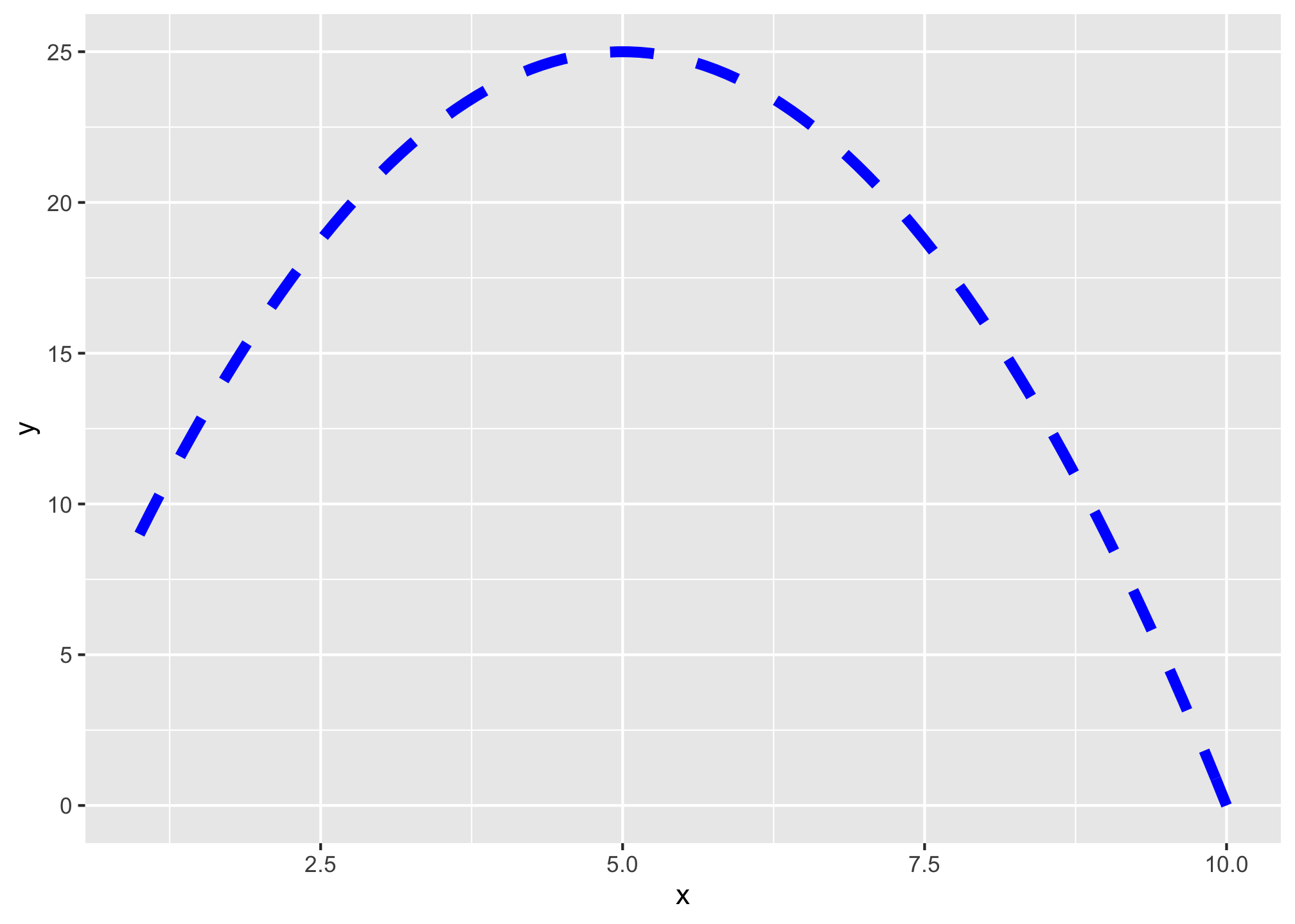
Bult-in Statistical Functions
There are some standard statistical distributions built into R. They require a combination of a specific prefix and a distribution.
Prefixes:
| Action/Type | Prefix |
|---|---|
| random draw | r |
| density (pdf) | d |
| cumulative density (cdf) | p |
| quantile (inverse cdf) | q |
Distributions:
| Distribution | Name in R |
|---|---|
| Normal | norm |
| Uniform | unif |
| Student’s t | t |
| Binomial | binom |
| Negative binomial | nbinom |
| Hypergeometric | hyper |
| Weibull | weibull |
| Beta | beta |
| Gamma | gamma |
Thus, what you want is a combination of the prefix and the distribution.
Some common examples:
- Take random draws from a normal distribution:
rnorm(n = 10, # take 10 draws from a normal distribution with:
      mean = 2, # mean of 2
      sd = 1) # sd of 1
## [1] 2.6070850 2.4363768 2.4640655 1.6825498 0.1926861 1.8054952 0.4379302
## [8] 2.9041258 2.5405607 1.3065504- Get probability of a random variable being less than or equal to a value (cdf) from a normal distribution:
# find probability of area to the LEFT of a number on pdf (note this = cdf of that number!)
pnorm(q = 80, # number is 80 from a distribution where:
      mean = 200, # mean is 100
      sd = 100, # sd is 100
      lower.tail = TRUE) # looking to the LEFT in lower tail
## [1] 0.1150697- Find the value of a distribution that is a specified percentile.
# find the 38th percentile value
qnorm(p = 0.38, # 38th percentile from a distribution where:
      mean = 200, # mean is 200
      sd = 100) # sd is 100
## [1] 169.4519Graphing Statistical Functions
You can also graph these commonly used statistical functions by setting fun = the named functions in your stat_function() layer. If you want to specify the mean and standard deviation, use args = list() to include the required arguments from the named function above (e.g. dnorm needs mean and sd).
ggplot(data = data.frame(x = -400:600))+
  aes(x = x)+
stat_function(fun = dnorm, args = list(mean = 200, sd = 200), color = "blue", size = 2, linetype = "dashed") 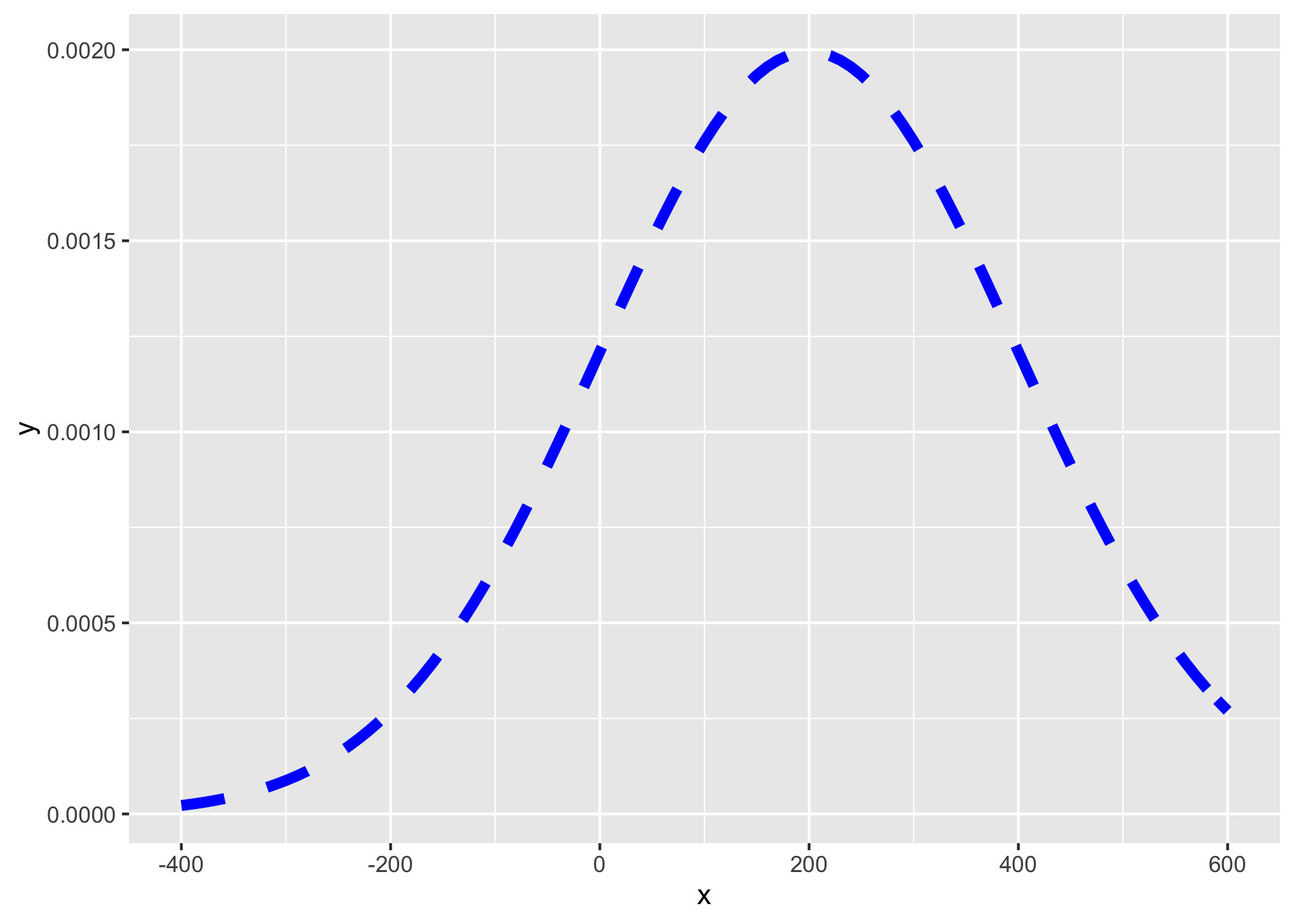
If you don’t include this, it will graph the standard distribution:
ggplot(data = data.frame(x = -4:4))+
  aes(x = x)+
stat_function(fun = dnorm, color = "blue", size = 2, linetype = "dashed") 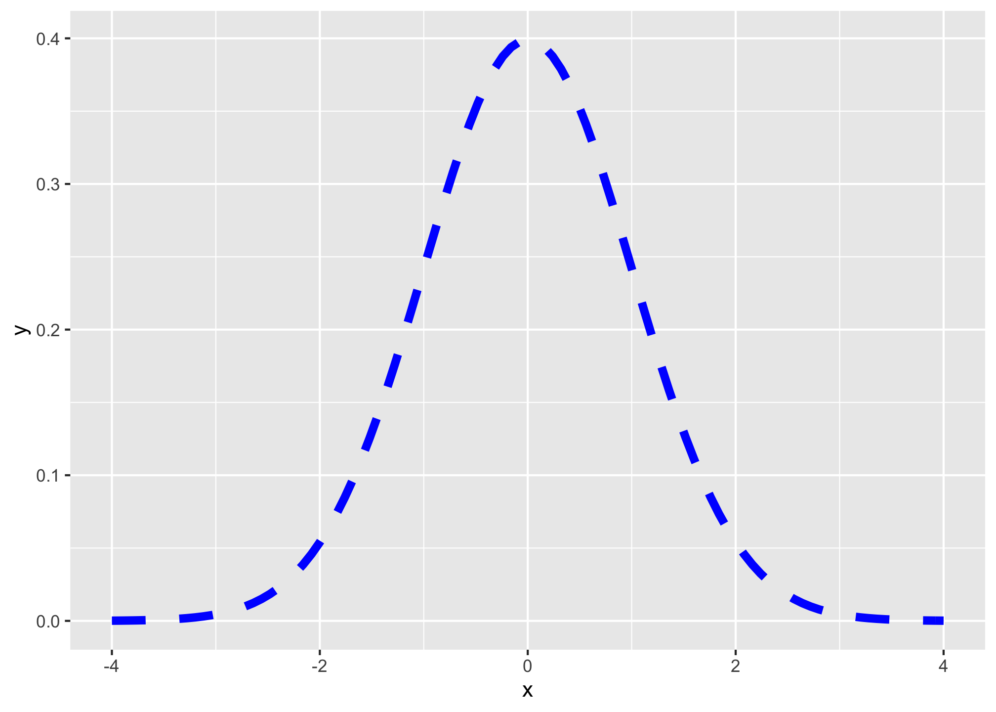
To add shading under a distribution, simply add a duplicate of the stat_function() layer, but add geom="area" to indicate the area beneath the function should be filled, and you can limit the domain of the fill with xlim=c(start,end), where start and end are the x-values for the endpoints of the fill.
# graph normal distribution and shade area between -2 and 2
ggplot(data = data.frame(x = -4:4))+
  aes(x = x)+
  stat_function(fun = dnorm, color = "blue", size = 2, linetype = "dashed")+
  stat_function(fun = dnorm, xlim = c(-2,2), geom = "area", fill = "green", alpha=0.5)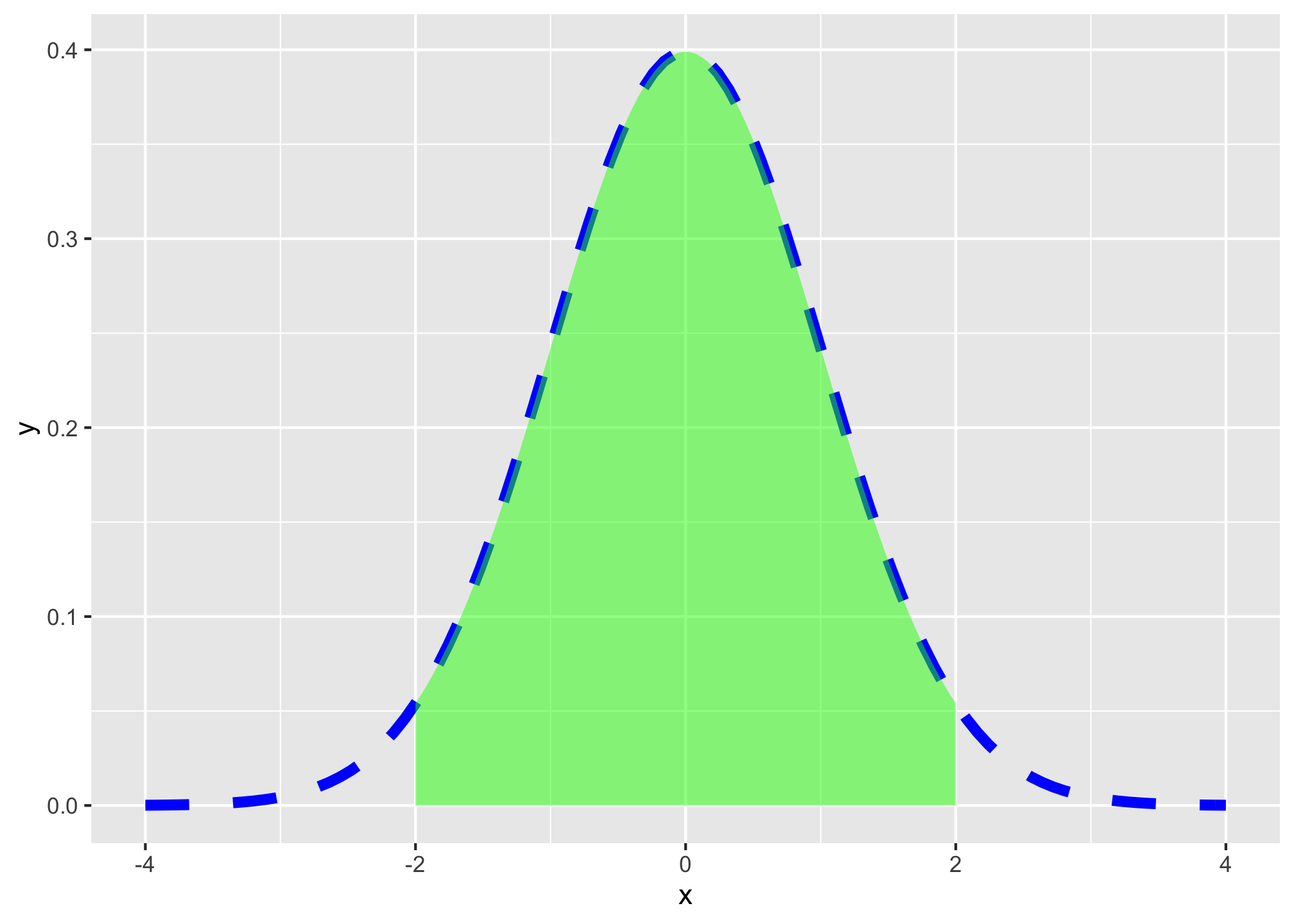
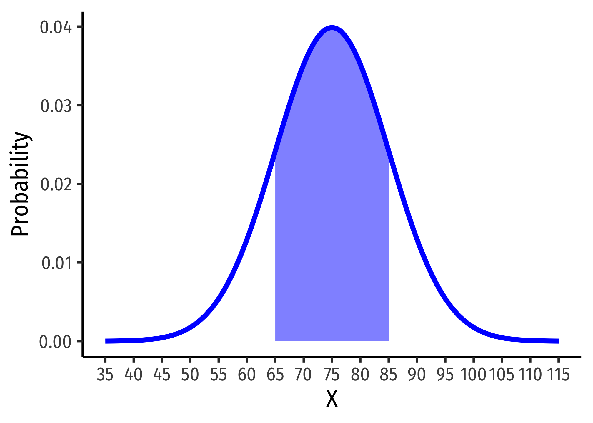
Hence, here is one graph from my slides:
ggplot(data = tibble(x=35:115))+
  aes(x = x)+
  stat_function(fun = dnorm, args = list(mean = 75, sd = 10), size = 2, color="blue")+
  stat_function(fun = dnorm, args = list(mean = 75, sd = 10), geom = "area", xlim = c(65,85), fill="blue", alpha=0.5)+
  labs(x = "X",
       y = "Probability")+
  scale_x_continuous(breaks = seq(35,115,5))+
  theme_classic(base_family = "Fira Sans Condensed",
           base_size=20)